PHY321: Classical Mechanics 1¶

Homework 1, due January 21 (midnight)

Date: Jan 11, 2022

Practicalities about homeworks and projects¶

You can work in groups (optimal groups are often 2-3 people) or by yourself. If you work as a group you can hand in one answer only if you wish. Remember to write your name(s)!
Homeworks (final version) are available approximately ten days before the deadline.
How do I(we) hand in? You can hand in the paper and pencil exercises as a scanned document. For this homework this applies to exercises 1-5. You should upload the scan to D2L. Alternatively, you can hand in everyhting (if you are ok with typing mathematical formulae using say Latex) as a jupyter notebook at D2L. The numerical exercise (exercise 6 here) should always be handed in as a jupyter notebook by the deadline at D2L.

Exercise 1 (12 pt), math reminder, properties of exponential function¶

The first exercise is meant to remind ourselves about properties of the exponential function and imaginary numbers. This is highly relevant later in this course when we start analyzing oscillatory motion and some wave mechanics. As physicists we should thus feel comfortable with expressions that include \(\exp{(\imath\omega t)}\). Here \(t\) could be interpreted as time and \(\omega\) as a frequency and \(\imath\) is the imaginary unit number.

1a (3pt): Perform Taylor expansions in powers of \(\omega t\) of the functions \(\cos{(\omega t)}\) and \(\sin{(\omega t)}\).
1b (3pt): Perform a Taylor expansion of \(\exp{(i\omega t)}\).
1c (3pt): Using parts (a) and (b) here, show that \(\exp{(\imath\omega t)}=\cos{(\omega t)}+\imath\sin{(\omega t)}\).
1d (3pt): Show that \(\ln{(−1)} = \imath\pi\).

Exercise 2 (12 pt), Vector algebra¶

2a (6pt) One of the many uses of the scalar product is to find the angle between two given vectors. Find the angle between the vectors \(\boldsymbol{a}=(1,2,4)\) and \(\boldsymbol{b}=(4,2,1)\) by evaluating their scalar product.
2b (6pt) For a cube with sides of length 1, one vertex at the origin, and sides along the \(x\), \(y\), and \(z\) axes, the vector of the body diagonal from the origin can be written \(\boldsymbol{a}=(1, 1, 1)\) and the vector of the face diagonal in the \(xy\) plane from the origin is \(\boldsymbol{b}=(1,1,0)\). Find first the lengths of the body diagonal and the face diagonal. Use then part (2a) to find the angle between the body diagonal and the face diagonal.

Exercise 3 (10 pt), More vector mathematics¶

3a (5pt) Show (using the fact that multiplication of reals is distributive) that \(\boldsymbol{a}(\boldsymbol{b}+\boldsymbol{c})=\boldsymbol{a}\boldsymbol{b}+\boldsymbol{a}\boldsymbol{c}\).
3b (5pt) Show that (using product rule for differentiating reals) \(\frac{d}{dt}(\boldsymbol{a}\boldsymbol{b})=\boldsymbol{a}\frac{d\boldsymbol{b}}{dt}+\boldsymbol{b}\frac{d\boldsymbol{a}}{dt}\)

Exercise 4 (10 pt), Algebra of cross products¶

4a (5pt) Show that the cross products are distribuitive \(\boldsymbol{a}\times(\boldsymbol{b}+\boldsymbol{c})=\boldsymbol{a}\times\boldsymbol{b}+\boldsymbol{a}\times\boldsymbol{c}\).
4b (5pt) Show that \(\frac{d}{dt}(\boldsymbol{a}\times\boldsymbol{b})=\boldsymbol{a}\times\frac{d\boldsymbol{b}}{dt}+\frac{d\boldsymbol{a}}{dt}\times \boldsymbol{b}\). Be careful with the order of factors

Exercise 5 (10 pt), Area of triangle and law of sines¶

Exercise 1.18 in the textbook of Taylor, Classical Mechanics. Part (1.18a) gives 5pt and part (1.18b) gives also 5pt.

Exercise 6 (40pt), Numerical elements, getting started with some simple data¶

This exercise should be handed in as a jupyter-notebook at D2L. Remember to write your name(s).

Our first numerical attempt will involve reading data from file or just setting up two vectors, one for position and one for time. Our data are from Usain Bolt’s world record 100m during the olympic games in Beijing in 2008. The data show the time used in units of 10m (see below). Before we however venture into this, we need to repeat some basic Python syntax with an emphasis on

basic Python syntax for arrays
define and operate on vectors and matrices in Python
create plots for motion in 1D space

For more information, see the introductory slides. Here are some of the basic packages we will be using this week

%matplotlib inline

import numpy as np 
import matplotlib.pyplot as plt
%matplotlib inline

The first exercise here deals with simply getting familiar with vectors and matrices.

We will be working with vectors and matrices to get you familiar with them

Initalize two three-dimensional \(xyz\) vectors in the below cell using np.array([x,y,z]). Vectors are represented through arrays in python
V1 should have x1=1, y1 =2, and z1=3.
Vector 2 should have x2=4, y2=5, and z2=6.
Print both vectors to make sure your code is working properly.

V1 = np.array([1,2,3])
V2 = np.array([4,5,6])
print("V1: ", V1)
print("V2: ", V2)

V1:  [1 2 3]
V2:  [4 5 6]

If this is not too familiar, here’s a useful link for creating vectors in python https://docs.scipy.org/doc/numpy-1.13.0/user/basics.creation.html. Alternatively, look up the introductory slides.

Now lets do some basic mathematics with vectors.

Compute and print the following, and double check with hand calculations:

6a (2pt) Calculate \(\boldsymbol{V}_1-\boldsymbol{V}_2\).
6b (2pt) Calculate \(\boldsymbol{V}_2-\boldsymbol{V}_1\).
6c (2pt) Calculate the dot product \(\boldsymbol{V}_1\boldsymbol{V}_2\).
6d (2pt) Calculate the cross product \(\boldsymbol{V}_1\times\boldsymbol{V}_2\).

Here is some useful explanation on numpy array operations if you feel a bit confused by what is happening, see https://www.pluralsight.com/guides/overview-basic-numpy-operations.

The following code prints the first two exercises

print(V1-V2)
print(V2-V1)

[-3 -3 -3]
[3 3 3]

For the dot product of V1 and V2 below we can use the dot function of numpy as follows

print(V1.dot(V2))

As a small challenge try to write your own function for the dot product of two vectors.

Matrices can be created in a similar fashion in python. In this language we can work with them through the package numpy (which we have already imported)

M1 = np.matrix([[1,2,3],
             [4,5,6],
             [7,8,9]])
M2 = np.matrix([[1,2],
             [3,4],
             [5,6]])
M3 = np.matrix([[9,8,7],
             [4,5,6],
             [7,6,9]])

Matrices can be added in the same way vectors are added in python as shown here

print("M1+M3: ", M1+M3)

M1+M3:  [[10 10 10]
 [ 8 10 12]
 [14 14 18]]

What happens if we try to do \(M1+M2\)?

That’s enough vectors and matrices for now. Let’s move on to some physics problems! Yes, the actual subject we are studying for.

We can opt for two different ways of handling the data. The data is listed in the table here and represents the total time Usain Bolt used in steps of 10 meters of distance. The label \(i\) is just a counter and we start from zero since Python arrays are by default set from zero. The variable \(t\) is time in seconds and \(x\) is the position in meters.

i	0	1	2	3	4	5	6	7	8	9
x[m]	10	20	30	40	50	60	70	80	90	100
t[s]	1.85	2.87	3.78	4.65	5.50	6.32	7.14	7.96	8.79	9.69

6e (6pt) You can here make a file with the above data and read them in and set up two vectors, one for time and one for position. Alternatively, you can just set up these two vectors directly and define two vectors in your Python code.

The following example code may help here

# we just initialize time and position
x = np.array([10.0, 20.0, 30.0, 40.0, 50.0, 60.0, 70.0, 80.0, 90.0, 100.0])
t = np.array([1.85, 2.87, 3.78, 4.65, 5.50, 6.32, 7.14, 7.96, 8.79, 9.69])
plt.plot(t,x, color='black')
plt.xlabel("Time t[s]")
plt.ylabel("Position x[m]")
plt.title("Usain Bolt's world record run")
plt.show()

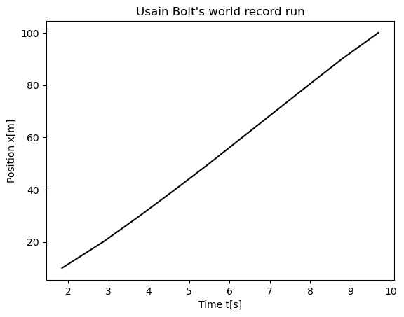
6f (6pt) Plot the position as function of time
6g (10pt) Compute thereafter the mean velocity for every interval \(i\) and the total velocity (from \(i=0\) to the given interval \(i\)) for each interval and plot these two quantities as function of time. Comment your results.
6h (10pt) Finally, compute and plot the mean acceleration for each interval and the total acceleration. Again, comment your results. Can you see whether he slowed down during the last meters?

Classical mechanics

PHY321: Classical Mechanics 1

Contents