Simple Motion problems and Reminder on Newton’s Laws
Contents
3. Simple Motion problems and Reminder on Newton’s Laws
3.1. Basic Steps of Scientific Investigations
An overarching aim in this course is to give you a deeper understanding of the scientific method. The problems we study will all involve cases where we can apply classical mechanics. In our previous material we already assumed that we had a model for the motion of an object. Alternatively we could have data from experiment (like Usain Bolt’s 100m world record run in 2008). Or we could have performed ourselves an experiment and we want to understand which forces are at play and whether these forces can be understood in terms of fundamental forces.
Our first step consists in identifying the problem. What we sketch here may include a mix of experiment and theoretical simulations, or just experiment or only theory.
3.1.1. Identifying our System
Here we can ask questions like
What kind of object is moving
What kind of data do we have
How do we measure position, velocity, acceleration etc
Which initial conditions influence our system
Other aspects which allow us to identify the system
3.1.2. Defining a Model
With our eventual data and observations we would now like to develop a model for the system. In the end we want obviously to be able to understand which forces are at play and how they influence our specific system. That is, can we extract some deeper insights about a system?
We need then to
Find the forces that act on our system
Introduce models for the forces
Identify the equations which can govern the system (Newton’s second law for example)
More elements we deem important for defining our model
3.1.3. Solving the Equations
With the model at hand, we can then solve the equations. In classical mechanics we normally end up with solving sets of coupled ordinary differential equations or partial differential equations.
Using Newton’s second law we have equations of the type \(\boldsymbol{F}=m\boldsymbol{a}=md\boldsymbol{v}/dt\)
We need to define the initial conditions (typically the initial velocity and position as functions of time) and/or initial conditions and boundary conditions
The solution of the equations give us then the position, the velocity and other time-dependent quantities which may specify the motion of a given object.
We are not yet done. With our lovely solvers, we need to start thinking.
3.1.4. Analyze
Now it is time to ask the big questions. What do our results mean? Can we give a simple interpretation in terms of fundamental laws? What do our results mean? Are they correct? Thus, typical questions we may ask are
Are our results for say \(\boldsymbol{r}(t)\) valid? Do we trust what we did? Can you validate and verify the correctness of your results?
Evaluate the answers and their implications
Compare with experimental data if possible. Does our model make sense?
and obviously many other questions.
The analysis stage feeds back to the first stage. It may happen that the data we had were not good enough, there could be large statistical uncertainties. We may need to collect more data or perhaps we did a sloppy job in identifying the degrees of freedom.
All these steps are essential elements in a scientific enquiry. Hopefully, through a mix of numerical simulations, analytical calculations and experiments we may gain a deeper insight about the physics of a specific system.
3.2. Newton’s Laws
Let us now remind ourselves of Newton’s laws, since these are the laws of motion we will study in this course.
When analyzing a physical system we normally start with distinguishing between the object we are studying (we will label this in more general terms as our system) and how this system interacts with the environment (which often means everything else!)
In our investigations we will thus analyze a specific physics problem in terms of the system and the environment. In doing so we need to identify the forces that act on the system and assume that the forces acting on the system must have a source, an identifiable cause in the environment.
A force acting on for example a falling object must be related to an interaction with something in the environment. This also means that we do not consider internal forces. The latter are forces between one part of the object and another part. In this course we will mainly focus on external forces.
Forces are either contact forces or long-range forces.
Contact forces, as evident from the name, are forces that occur at the contact between the system and the environment. Well-known long-range forces are the gravitional force and the electromagnetic force.
In order to set up the forces which act on an object, the following steps may be useful
Divide the problem into system and environment.
Draw a figure of the object and everything in contact with the object.
Draw a closed curve around the system.
Find contact points—these are the points where contact forces may act.
Give names and symbols to all the contact forces.
Identify the long-range forces.
Make a drawing of the object. Draw the forces as arrows, vectors, starting from where the force is acting. The direction of the vector(s) indicates the (positive) direction of the force. Try to make the length of the arrow indicate the relative magnitude of the forces.
Draw in the axes of the coordinate system. It is often convenient to make one axis parallel to the direction of motion. When you choose the direction of the axis you also choose the positive direction for the axis.
Newton’s second law of motion: The force \(\boldsymbol{F}\) on an object of inertial mass \(m\) is related to the acceleration a of the object through
where \(\boldsymbol{a}\) is the acceleration.
Newton’s laws of motion are laws of nature that have been found by experimental investigations and have been shown to hold up to continued experimental investigations. Newton’s laws are valid over a wide range of length- and time-scales. We use Newton’s laws of motion to describe everything from the motion of atoms to the motion of galaxies.
The second law is a vector equation with the acceleration having the same direction as the force. The acceleration is proportional to the force via the mass \(m\) of the system under study.
Newton’s second law introduces a new property of an object, the so-called inertial mass \(m\). We determine the inertial mass of an object by measuring the acceleration for a given applied force.
3.2.1. Then the First Law
What happens if the net external force on a body is zero? Applying Newton’s second law, we find:
which gives using the definition of the acceleration
The acceleration is zero, which means that the velocity of the object is constant. This is often referred to as Newton’s first law. An object in a state of uniform motion tends to remain in that state unless an external force changes its state of motion. Why do we need a separate law for this? Is it not simply a special case of Newton’s second law? Yes, Newton’s first law can be deduced from the second law as we have illustrated. However, the first law is often used for a different purpose: Newton’s First Law tells us about the limit of applicability of Newton’s Second law. Newton’s Second law can only be used in reference systems where the First law is obeyed. But is not the First law always valid? No! The First law is only valid in reference systems that are not accelerated. If you observe the motion of a ball from an accelerating car, the ball will appear to accelerate even if there are no forces acting on it. We call systems that are not accelerating inertial systems, and Newton’s first law is often called the law of inertia. Newton’s first and second laws of motion are only valid in inertial systems.
A system is an inertial system if it is not accelerated. It means that the reference system must not be accelerating linearly or rotating. Unfortunately, this means that most systems we know are not really inertial systems. For example, the surface of the Earth is clearly not an inertial system, because the Earth is rotating. The Earth is also not an inertial system, because it ismoving in a curved path around the Sun. However, even if the surface of the Earth is not strictly an inertial system, it may be considered to be approximately an inertial system for many laboratory-size experiments.
3.2.2. And finally the Third Law
If there is a force from object A on object B, there is also a force from object B on object A. This fundamental principle of interactions is called Newton’s third law. We do not know of any force that do not obey this law: All forces appear in pairs. Newton’s third law is usually formulated as: For every action there is an equal and opposite reaction.
3.3. Falling baseball in one dimension
We anticipate the mathematical model to come and assume that we have a model for the motion of a falling baseball without air resistance. Our system (the baseball) is at an initial height \(y_0\) (which we will specify in the program below) at the initial time \(t_0=0\). In our program example here we will plot the position in steps of \(\Delta t\) up to a final time \(t_f\). The mathematical formula for the position \(y(t)\) as function of time \(t\) is
where \(g=9.80665=0.980655\times 10^1\)m/s\(^2\) is a constant representing the standard acceleration due to gravity. We have here adopted the conventional standard value. This does not take into account other effects, such as buoyancy or drag. Furthermore, we stop when the ball hits the ground, which takes place at
which gives us a final time \(t_f=\sqrt{2y_0/g}\).
As of now we simply assume that we know the formula for the falling object. Afterwards, we will derive it.
We start with preparing folders for storing our calculations, figures and if needed, specific data files we use as input or output files.
%matplotlib inline

# Common imports
import numpy as np
import pandas as pd
import matplotlib.pyplot as plt
import os

# Where to save the figures and data files
PROJECT_ROOT_DIR = "Results"
FIGURE_ID = "Results/FigureFiles"
DATA_ID = "DataFiles/"

if not os.path.exists(PROJECT_ROOT_DIR):
    os.mkdir(PROJECT_ROOT_DIR)

if not os.path.exists(FIGURE_ID):
    os.makedirs(FIGURE_ID)

if not os.path.exists(DATA_ID):
    os.makedirs(DATA_ID)

def image_path(fig_id):
    return os.path.join(FIGURE_ID, fig_id)

def data_path(dat_id):
    return os.path.join(DATA_ID, dat_id)

def save_fig(fig_id):
    plt.savefig(image_path(fig_id) + ".png", format='png')

#in case we have an input file we wish to read in
#infile = open(data_path("MassEval2016.dat"),'r')
You could also define a function for making our plots. You can obviously avoid this and simply set up various matplotlib commands every time you need them. You may however find it convenient to collect all such commands in one function and simply call this function.
from pylab import plt, mpl
plt.style.use('seaborn')
mpl.rcParams['font.family'] = 'serif'

def MakePlot(x,y, styles, labels, axlabels):
    plt.figure(figsize=(10,6))
    for i in range(len(x)):
        plt.plot(x[i], y[i], styles[i], label = labels[i])
        plt.xlabel(axlabels[0])
        plt.ylabel(axlabels[1])
    plt.legend(loc=0)
Thereafter we start setting up the code for the falling object.
%matplotlib inline
import matplotlib.patches as mpatches

g = 9.80655 #m/s^2
y_0 = 10.0 # initial position in meters
DeltaT = 0.1  # time step
# final time when y = 0, t = sqrt(2*10/g)
tfinal = np.sqrt(2.0*y_0/g)
#set up arrays
t = np.arange(0,tfinal,DeltaT)
y =y_0 -g*.5*t**2
# Then make a nice printout in table form using Pandas
import pandas as pd
from IPython.display import display
data = {'t[s]': t,
        'y[m]': y
        }
RawData = pd.DataFrame(data)
display(RawData)
plt.style.use('ggplot')
plt.figure(figsize=(8,8))
plt.scatter(t, y, color = 'b')
blue_patch = mpatches.Patch(color = 'b', label = 'Height y as function of  time t')
plt.legend(handles=[blue_patch])
plt.xlabel("t[s]")
plt.ylabel("y[m]")
save_fig("FallingBaseball")
plt.show()
| t[s] | y[m] | |
|---|---|---|
| 0 | 0.0 | 10.000000 |
| 1 | 0.1 | 9.950967 |
| 2 | 0.2 | 9.803869 |
| 3 | 0.3 | 9.558705 |
| 4 | 0.4 | 9.215476 |
| 5 | 0.5 | 8.774181 |
| 6 | 0.6 | 8.234821 |
| 7 | 0.7 | 7.597395 |
| 8 | 0.8 | 6.861904 |
| 9 | 0.9 | 6.028347 |
| 10 | 1.0 | 5.096725 |
| 11 | 1.1 | 4.067037 |
| 12 | 1.2 | 2.939284 |
| 13 | 1.3 | 1.713465 |
| 14 | 1.4 | 0.389581 |
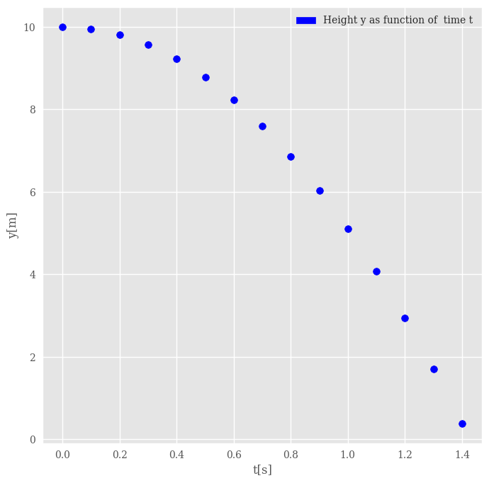
Here we used pandas (see below) to systemize the output of the position as function of time.
We define now the average velocity as
In the code we have set the time step \(\Delta t\) to a given value. We could define it in terms of the number of points \(n\) as
Since we have discretized the variables, we introduce the counter \(i\) and let \(y(t)\rightarrow y(t_i)=y_i\) and \(t\rightarrow t_i\) with \(i=0,1,\dots, n\). This gives us the following shorthand notations that we will use for the rest of this course. We define
This applies to other variables which depend on say time. Examples are the velocities, accelerations, momenta etc. Furthermore we use the shorthand
3.3.1. Compact equations
We can then rewrite in a more compact form the average velocity as
The velocity is defined as the change in position per unit time. In the limit \(\Delta t \rightarrow 0\) this defines the instantaneous velocity, which is nothing but the slope of the position at a time \(t\). We have thus
Similarly, we can define the average acceleration as the change in velocity per unit time as
resulting in the instantaneous acceleration
A note on notations: When writing for example the velocity as \(v(t)\) we are then referring to the continuous and instantaneous value. A subscript like \(v_i\) refers always to the discretized values.
We can rewrite the instantaneous acceleration as
This forms the starting point for our definition of forces later. It is a famous second-order differential equation. If the acceleration is constant we can now recover the formula for the falling ball we started with. The acceleration can depend on the position and the velocity. To be more formal we should then write the above differential equation as
With given initial conditions for \(y(t_0)\) and \(v(t_0)\) we can then integrate the above equation and find the velocities and positions at a given time \(t\).
If we multiply with mass, we have one of the famous expressions for Newton’s second law,
where \(F\) is the force acting on an object with mass \(m\). We see that it also has the right dimension, mass times length divided by time squared. We will come back to this soon.
3.3.2. Integrating our equations
Formally we can then, starting with the acceleration (suppose we have measured it, how could we do that?) compute say the height of a building. To see this we perform the following integrations from an initial time \(t_0\) to a given time \(t\)
or as
When we know the velocity as function of time, we can find the position as function of time starting from the defintion of velocity as the derivative with respect to time, that is we have
or as
These equations define what is called the integration method for finding the position and the velocity as functions of time. There is no loss of generality if we extend these equations to more than one spatial dimension.
Let us compute the velocity using the constant value for the acceleration given by \(-g\). We have
Using our initial time as \(t_0=0\)s and setting the initial velocity \(v(t_0)=v_0=0\)m/s we get when integrating
The more general case is
We can then integrate the velocity and obtain the final formula for the position as function of time through
With \(y_0=10\)m and \(t_0=0\)s, we obtain the equation we started with
3.3.3. Computing the averages
After this mathematical background we are now ready to compute the mean velocity using our data.
# Now we can compute the mean velocity using our data
# We define first an array Vaverage
n = np.size(t)
Vaverage = np.zeros(n)
for i in range(1,n-1):
    Vaverage[i] = (y[i+1]-y[i])/DeltaT
# Now we can compute the mean accelearatio using our data
# We define first an array Aaverage
n = np.size(t)
Aaverage = np.zeros(n)
Aaverage[0] = -g
for i in range(1,n-1):
    Aaverage[i] = (Vaverage[i+1]-Vaverage[i])/DeltaT
data = {'t[s]': t,
        'y[m]': y,
        'v[m/s]': Vaverage,
        'a[m/s^2]': Aaverage
        }
NewData = pd.DataFrame(data)
display(NewData[0:n-2])
| t[s] | y[m] | v[m/s] | a[m/s^2] | |
|---|---|---|---|---|
| 0 | 0.0 | 10.000000 | 0.000000 | -9.80655 |
| 1 | 0.1 | 9.950967 | -1.470982 | -9.80655 |
| 2 | 0.2 | 9.803869 | -2.451638 | -9.80655 |
| 3 | 0.3 | 9.558705 | -3.432292 | -9.80655 |
| 4 | 0.4 | 9.215476 | -4.412948 | -9.80655 |
| 5 | 0.5 | 8.774181 | -5.393602 | -9.80655 |
| 6 | 0.6 | 8.234821 | -6.374258 | -9.80655 |
| 7 | 0.7 | 7.597395 | -7.354913 | -9.80655 |
| 8 | 0.8 | 6.861904 | -8.335567 | -9.80655 |
| 9 | 0.9 | 6.028347 | -9.316222 | -9.80655 |
| 10 | 1.0 | 5.096725 | -10.296878 | -9.80655 |
| 11 | 1.1 | 4.067037 | -11.277533 | -9.80655 |
| 12 | 1.2 | 2.939284 | -12.258187 | -9.80655 |
Note that we don’t print the last values!
3.4. Including Air Resistance in our model
In our discussions till now of the falling baseball, we have ignored air resistance and simply assumed that our system is only influenced by the gravitational force. We will postpone the derivation of air resistance till later, after our discussion of Newton’s laws and forces.
For our discussions here it suffices to state that the accelerations is now modified to
where \(\vert v(t)\vert\) is the absolute value of the velocity and \(D\) is a constant which pertains to the specific object we are studying. Since we are dealing with motion in one dimension, we can simplify the above to
We can rewrite this as a differential equation
Using the integral equations discussed above we can integrate twice and obtain first the velocity as function of time and thereafter the position as function of time.
For this particular case, we can actually obtain an analytical solution for the velocity and for the position. Here we will first compute the solutions analytically, thereafter we will derive Euler’s method for solving these differential equations numerically.
For simplicity let us just write \(v(t)\) as \(v\). We have
We can solve this using the technique of separation of variables. We isolate on the left all terms that involve \(v\) and on the right all terms that involve time. We get then
We scale now the equation to the left by introducing a constant \(v_T=\sqrt{g/D}\). This constant has dimension length/time. Can you show this?
Next we integrate the left-hand side (lhs) from \(v_0=0\) m/s to \(v\) and the right-hand side (rhs) from \(t_0=0\) to \(t\) and obtain
We can reorganize these equations as
which gives us \(v\) as function of time
With the velocity we can then find the height \(y(t)\) by integrating yet another time, that is
This integral is a little bit trickier but we can look it up in a table over known integrals and we get
Alternatively we could have used the symbolic Python package Sympy (example will be inserted later).
In most cases however, we need to revert to numerical solutions.
3.5. Our first attempt at solving differential equations
Here we will try the simplest possible approach to solving the second-order differential equation
We rewrite it as two coupled first-order equations (this is a standard approach)
with initial condition \(y(t_0)=y_0\) and
with initial condition \(v(t_0)=v_0\).
Many of the algorithms for solving differential equations start with simple Taylor equations. If we now Taylor expand \(y\) and \(v\) around a value \(t+\Delta t\) we have
and
Using the fact that \(dy/dt = v\) and \(dv/dt=a\) and keeping only terms up to \(\Delta t\) we have
and
3.5.1. Discretizing our equations
Using our discretized versions of the equations with for example \(y_{i}=y(t_i)\) and \(y_{i\pm 1}=y(t_i+\Delta t)\), we can rewrite the above equations as (and truncating at \(\Delta t\))
and
These are the famous Euler equations (forward Euler).
To solve these equations numerically we start at a time \(t_0\) and simply integrate up these equations to a final time \(t_f\), The step size \(\Delta t\) is an input parameter in our code. You can define it directly in the code below as
DeltaT = 0.1
With a given final time tfinal we can then find the number of integration points via the ceil function included in the math package of Python as
#define final time, assuming that initial time is zero
from math import ceil
tfinal = 0.5
n = ceil(tfinal/DeltaT)
print(n)
5
The ceil function returns the smallest integer not less than the input in say
x = 21.15
print(ceil(x))
22
which in the case here is 22.
x = 21.75
print(ceil(x))
22
which also yields 22. The floor function in the math package is used to return the closest integer value which is less than or equal to the specified expression or value. Compare the previous result to the usage of floor
from math import floor
x = 21.75
print(floor(x))
21
Alternatively, we can define ourselves the number of integration(mesh) points. In this case we could have
n = 10
tinitial = 0.0
tfinal = 0.5
DeltaT = (tfinal-tinitial)/(n)
print(DeltaT)
0.05
Since we will set up one-dimensional arrays that contain the values of various variables like time, position, velocity, acceleration etc, we need to know the value of \(n\), the number of data points (or integration or mesh points). With \(n\) we can initialize a given array by setting all elelements to zero, as done here
# define array a
a = np.zeros(n)
print(a)
[0. 0. 0. 0. 0. 0. 0. 0. 0. 0.]
In the code here we implement this simple Eurler scheme choosing a value for \(D=0.0245\) m/s.
# Common imports
import numpy as np
import pandas as pd
from math import *
import matplotlib.pyplot as plt
import os

# Where to save the figures and data files
PROJECT_ROOT_DIR = "Results"
FIGURE_ID = "Results/FigureFiles"
DATA_ID = "DataFiles/"

if not os.path.exists(PROJECT_ROOT_DIR):
    os.mkdir(PROJECT_ROOT_DIR)

if not os.path.exists(FIGURE_ID):
    os.makedirs(FIGURE_ID)

if not os.path.exists(DATA_ID):
    os.makedirs(DATA_ID)

def image_path(fig_id):
    return os.path.join(FIGURE_ID, fig_id)

def data_path(dat_id):
    return os.path.join(DATA_ID, dat_id)

def save_fig(fig_id):
    plt.savefig(image_path(fig_id) + ".png", format='png')


g = 9.80655 #m/s^2
D = 0.00245 #m/s
DeltaT = 0.1
#set up arrays
tfinal = 0.5
n = ceil(tfinal/DeltaT)
# define scaling constant vT
vT = sqrt(g/D)
# set up arrays for t, a, v, and y and we can compare our results with analytical ones
t = np.zeros(n)
a = np.zeros(n)
v = np.zeros(n)
y = np.zeros(n)
yanalytic = np.zeros(n)
# Initial conditions
v[0] = 0.0  #m/s
y[0] = 10.0 #m
yanalytic[0] = y[0]
# Start integrating using Euler's method
for i in range(n-1):
    # expression for acceleration
    a[i] = -g + D*v[i]*v[i]
    # update velocity and position
    y[i+1] = y[i] + DeltaT*v[i]
    v[i+1] = v[i] + DeltaT*a[i]
    # update time to next time step and compute analytical answer
    t[i+1] = t[i] + DeltaT
    yanalytic[i+1] = y[0]-(vT*vT/g)*log(cosh(g*t[i+1]/vT))
    if ( y[i+1] < 0.0):
        break
a[n-1] = -g + D*v[n-1]*v[n-1]
data = {'t[s]': t,
        'y[m]': y-yanalytic,
        'v[m/s]': v,
        'a[m/s^2]': a
        }
NewData = pd.DataFrame(data)
display(NewData)
#finally we plot the data
fig, axs = plt.subplots(3, 1)
axs[0].plot(t, y, t, yanalytic)
axs[0].set_xlim(0, tfinal)
axs[0].set_ylabel('y and exact')
axs[1].plot(t, v)
axs[1].set_ylabel('v[m/s]')
axs[2].plot(t, a)
axs[2].set_xlabel('time[s]')
axs[2].set_ylabel('a[m/s^2]')
fig.tight_layout()
save_fig("EulerIntegration")
plt.show()
| t[s] | y[m] | v[m/s] | a[m/s^2] | |
|---|---|---|---|---|
| 0 | 0.0 | 0.000000 | 0.000000 | -9.806550 |
| 1 | 0.1 | 0.049031 | -0.980655 | -9.804194 |
| 2 | 0.2 | 0.098034 | -1.961074 | -9.797128 |
| 3 | 0.3 | 0.146963 | -2.940787 | -9.785362 |
| 4 | 0.4 | 0.195770 | -3.919323 | -9.768915 |
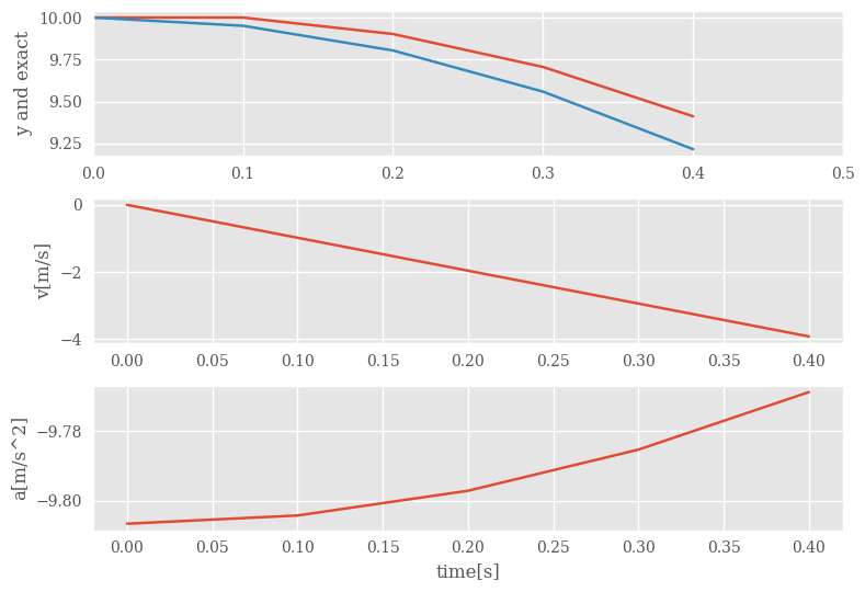
Try different values for \(\Delta t\) and study the difference between the exact solution and the numerical solution.
3.5.2. Simple extension, the Euler-Cromer method
The Euler-Cromer method is a simple variant of the standard Euler method. We use the newly updated velocity \(v_{i+1}\) as an input to the new position, that is, instead of
and
we use now the newly calculate for \(v_{i+1}\) as input to \(y_{i+1}\), that is we compute first
and then
Implementing the Euler-Cromer method yields a simple change to the previous code. We only need to change the following line in the loop over time steps
for i in range(n-1):
    # more codes in between here
    v[i+1] = v[i] + DeltaT*a[i]
    y[i+1] = y[i] + DeltaT*v[i+1]
    # more code
3.6. Air Resistance in One Dimension
Here we look at both a quadratic in velocity resistance and linear in velocity. But first we give a qualitative argument about the mathematical expression for the air resistance we used last Friday.
Air resistance tends to scale as the square of the velocity. This is in contrast to many problems chosen for textbooks, where it is linear in the velocity. The choice of a linear dependence is motivated by mathematical simplicity (it keeps the differential equation linear) rather than by physics. One can see that the force should be quadratic in velocity by considering the momentum imparted on the air molecules. If an object sweeps through a volume \(dV\) of air in time \(dt\), the momentum imparted on the air is
where \(v\) is the velocity of the object and \(\rho_m\) is the mass density of the air. If the molecules bounce back as opposed to stop you would double the size of the term. The opposite value of the momentum is imparted onto the object itself. Geometrically, the differential volume is
where \(A\) is the cross-sectional area and \(vdt\) is the distance the object moved in time \(dt\).
Plugging this into the expression above,
This is the force felt by the particle, and is opposite to its direction of motion. Now, because air doesn’t stop when it hits an object, but flows around the best it can, the actual force is reduced by a dimensionless factor \(c_W\), called the drag coefficient.
and the acceleration is
For a particle with initial velocity \(v_0\), one can separate the \(dt\) to one side of the equation, and move everything with \(v\)s to the other side. We did this in our discussion of simple motion and will not repeat it here.
On more general terms, for many systems, e.g. an automobile, there are multiple sources of resistance. In addition to wind resistance, where the force is proportional to \(v^2\), there are dissipative effects of the tires on the pavement, and in the axel and drive train. These other forces can have components that scale proportional to \(v\), and components that are independent of \(v\). Those independent of \(v\), e.g. the usual \(f=\mu_K N\) frictional force you consider in your first Physics courses, only set in once the object is actually moving. As speeds become higher, the \(v^2\) components begin to dominate relative to the others. For automobiles at freeway speeds, the \(v^2\) terms are largely responsible for the loss of efficiency. To travel a distance \(L\) at fixed speed \(v\), the energy/work required to overcome the dissipative forces are \(fL\), which for a force of the form \(f=\alpha v^n\) becomes
For \(n=0\) the work is independent of speed, but for the wind resistance, where \(n=2\), slowing down is essential if one wishes to reduce fuel consumption. It is also important to consider that engines are designed to be most efficient at a chosen range of power output. Thus, some cars will get better mileage at higher speeds (They perform better at 50 mph than at 5 mph) despite the considerations mentioned above.
As an example of Newton’s Laws we consider projectile motion (or a falling raindrop or a ball we throw up in the air) with a drag force. Even though air resistance is largely proportional to the square of the velocity, we will consider the drag force to be linear to the velocity, \(\boldsymbol{F}=-m\gamma\boldsymbol{v}\), for the purposes of this exercise.
Such a dependence can be extracted from experimental data for objects moving at low velocities, see for example Malthe-Sørenssen chapter 5.6.
We will here focus on a two-dimensional problem.
The acceleration for a projectile moving upwards, \(\boldsymbol{a}=\boldsymbol{F}/m\), becomes
and \(\gamma\) has dimensions of inverse time.
If you on the other hand have a falling raindrop, how do these equations change? See for example Figure 2.1 in Taylor. Let us stay with a ball which is thrown up in the air at \(t=0\).
3.7. Ways of solving these equations
We will go over two different ways to solve this equation. The first by direct integration, and the second as a differential equation. To do this by direct integration, one simply multiplies both sides of the equations above by \(dt\), then divide by the appropriate factors so that the \(v\)s are all on one side of the equation and the \(dt\) is on the other. For the \(x\) motion one finds an easily integrable equation,
This is very much the result you would have written down by inspection. For the \(y\)-component of the velocity,
Whereas \(v_x\) starts at some value and decays exponentially to zero, \(v_y\) decays exponentially to the terminal velocity, \(v_t=-g/\gamma\).
Although this direct integration is simpler than the method we invoke below, the method below will come in useful for some slightly more difficult differential equations in the future. The differential equation for \(v_x\) is straight-forward to solve. Because it is first order there is one arbitrary constant, \(A\), and by inspection the solution is
The arbitrary constants for equations of motion are usually determined by the initial conditions, or more generally boundary conditions. By inspection \(A=v_{0x}\), the initial \(x\) component of the velocity.
3.8. Differential Equations, contn
The differential equation for \(v_y\) is a bit more complicated due to the presence of \(g\). Differential equations where all the terms are linearly proportional to a function, in this case \(v_y\), or to derivatives of the function, e.g., \(v_y\), \(dv_y/dt\), \(d^2v_y/dt^2\cdots\), are called linear differential equations. If there are terms proportional to \(v^2\), as would happen if the drag force were proportional to the square of the velocity, the differential equation is not longer linear. Because this expression has only one derivative in \(v\) it is a first-order linear differential equation. If a term were added proportional to \(d^2v/dt^2\) it would be a second-order differential equation. In this case we have a term completely independent of \(v\), the gravitational acceleration \(g\), and the usual strategy is to first rewrite the equation with all the linear terms on one side of the equal sign,
Now, the solution to the equation can be broken into two parts. Because this is a first-order differential equation we know that there will be one arbitrary constant. Physically, the arbitrary constant will be determined by setting the initial velocity, though it could be determined by setting the velocity at any given time. Like most differential equations, solutions are not “solved”. Instead, one guesses at a form, then shows the guess is correct. For these types of equations, one first tries to find a single solution, i.e. one with no arbitrary constants. This is called the {\it particular} solution, \(y_p(t)\), though it should really be called “a” particular solution because there are an infinite number of such solutions. One then finds a solution to the {\it homogenous} equation, which is the equation with zero on the right-hand side,
Homogenous solutions will have arbitrary constants.
The particular solution will solve the same equation as the original general equation
However, we don’t need find one with arbitrary constants. Hence, it is called a particular solution.
The sum of the two,
is a solution of the total equation because of the linear nature of the differential equation. One has now found a general solution encompassing all solutions, because it both satisfies the general equation (like the particular solution), and has an arbitrary constant that can be adjusted to fit any initial condition (like the homogeneous solution). If the equations were not linear, that is if there were terms such as \(v_y^2\) or \(v_y\dot{v}_y\), this technique would not work.
Returning to the example above, the homogenous solution is the same as that for \(v_x\), because there was no gravitational acceleration in that case,
In this case a particular solution is one with constant velocity,
Note that this is the terminal velocity of a particle falling from a great height. The general solution is thus,
and one can find \(B\) from the initial velocity,
Plugging in the expression for \(B\) gives the \(y\) motion given the initial velocity,
It is easy to see that this solution has \(v_y=v_{0y}\) when \(t=0\) and \(v_y=-g/\gamma\) when \(t\rightarrow\infty\).
One can also integrate the two equations to find the coordinates \(x\) and \(y\) as functions of \(t\),
If the question was to find the position at a time \(t\), we would be finished. However, the more common goal in a projectile equation problem is to find the range, i.e. the distance \(x\) at which \(y\) returns to zero. For the case without a drag force this was much simpler. The solution for the \(y\) coordinate would have been \(y=v_{0y}t-gt^2/2\). One would solve for \(t\) to make \(y=0\), which would be \(t=2v_{0y}/g\), then plug that value for \(t\) into \(x=v_{0x}t\) to find \(x=2v_{0x}v_{0y}/g=v_0\sin(2\theta_0)/g\). One follows the same steps here, except that the expression for \(y(t)\) is more complicated. Searching for the time where \(y=0\), and we get
This cannot be inverted into a simple expression \(t=\cdots\). Such expressions are known as “transcendental equations”, and are not the rare instance, but are the norm. In the days before computers, one might plot the right-hand side of the above graphically as a function of time, then find the point where it crosses zero.
Now, the most common way to solve for an equation of the above type would be to apply Newton’s method numerically. This involves the following algorithm for finding solutions of some equation \(F(t)=0\).
First guess a value for the time, \(t_{\rm guess}\).
Calculate \(F\) and its derivative, \(F(t_{\rm guess})\) and \(F'(t_{\rm guess})\).
Unless you guessed perfectly, \(F\ne 0\), and assuming that \(\Delta F\approx F'\Delta t\), one would choose
\(\Delta t=-F(t_{\rm guess})/F'(t_{\rm guess})\).
Now repeat step 1, but with \(t_{\rm guess}\rightarrow t_{\rm guess}+\Delta t\).
If the \(F(t)\) were perfectly linear in \(t\), one would find \(t\) in one step. Instead, one typically finds a value of \(t\) that is closer to the final answer than \(t_{\rm guess}\). One breaks the loop once one finds \(F\) within some acceptable tolerance of zero. A program to do this will be added shortly.
3.9. Motion in a Magnetic Field
Another example of a velocity-dependent force is magnetism,
For a uniform field in the \(z\) direction \(\boldsymbol{B}=B\hat{z}\), the force can only have \(x\) and \(y\) components,
The differential equations are
One can solve the equations by taking time derivatives of either equation, then substituting into the other equation,
The solution to these equations can be seen by inspection,
One can integrate the equations to find the positions as a function of time,
The trajectory is a circle centered at \(x_0,y_0\) with amplitude \(A\) rotating in the clockwise direction.
The equations of motion for the \(z\) motion are
which leads to
Added onto the circle, the motion is helical.
Note that the kinetic energy,
is constant. This is because the force is perpendicular to the velocity, so that in any differential time element \(dt\) the work done on the particle \(\boldsymbol{F}\cdot{dr}=dt\boldsymbol{F}\cdot{v}=0\).
One should think about the implications of a velocity dependent force. Suppose one had a constant magnetic field in deep space. If a particle came through with velocity \(v_0\), it would undergo cyclotron motion with radius \(R=v_0/\omega_c\). However, if it were still its motion would remain fixed. Now, suppose an observer looked at the particle in one reference frame where the particle was moving, then changed their velocity so that the particle’s velocity appeared to be zero. The motion would change from circular to fixed. Is this possible?
The solution to the puzzle above relies on understanding relativity. Imagine that the first observer believes \(\boldsymbol{B}\ne 0\) and that the electric field \(\boldsymbol{E}=0\). If the observer then changes reference frames by accelerating to a velocity \(\boldsymbol{v}\), in the new frame \(\boldsymbol{B}\) and \(\boldsymbol{E}\) both change. If the observer moved to the frame where the charge, originally moving with a small velocity \(v\), is now at rest, the new electric field is indeed \(\boldsymbol{v}\times\boldsymbol{B}\), which then leads to the same acceleration as one had before. If the velocity is not small compared to the speed of light, additional \(\gamma\) factors come into play, \(\gamma=1/\sqrt{1-(v/c)^2}\). Relativistic motion will not be considered in this course.
3.10. Summarizing the various motion problems
The examples we have discussed above were included in order to illustrate various methods (which depend on the specific problem) to find the solutions of the equations of motion. We have solved the equations of motion in the following ways:
Solve the differential equations analytically.
We did this for example with the following object in one or two dimensions or the sliding block. Here we had for example an equation set like
and
and \(\gamma\) has dimension of inverse time.
We could also in case we can separate the degrees of freedom integrate. Take for example one of the equations in the previous slide
which we can rewrite in terms of a left-hand side which depends only on the velocity and a right-hand side which depends only on time
Integrating we have (since we can separate \(v_x\) and \(t\))
where \(v_f\) is the velocity at a final time and \(t_f\) is the final time. In this case we found, after having integrated the above two sides that
Finally, using for example Euler’s method, we can solve the differential equations numerically. If we can compare our numerical solutions with analytical solutions, we have an extra check of our numerical approaches.
3.11. Exercises
3.11.1. Electron moving into an electric field
An electron is sent through a varying electrical field. Initially, the electron is moving in the \(x\)-direction with a velocity \(v_x = 100\) m/s. The electron enters the field when it passes the origin. The field varies with time, causing an acceleration of the electron that varies in time
or if we replace \(\boldsymbol{e}_y\) with \(\boldsymbol{e}_2\) (the unit vectors in the \(y\)-direction) we have
Note that the velocity in the \(x\)-direction is a constant and is not affected by the force which acts only in the \(y\)-direction. This means that we can decouple the two degrees of freedom and skip the vector symbols. We have then a constant velocity in the \(x\)-direction
and integrating up the acceleration in the \(y\)-direction (and using that the initial time \(t_0=0\)) we get
Find the position as a function of time for the electron.
We integrate again in the \(x\)-direction
and in the \(y\)-direction (remember that these two degrees of freedom don’t depend on each other) we get
The field is only acting inside a box of length \(L = 2m\).
How long time is the electron inside the field?
If we use the equation for the \(x\)-direction (the length of the box), we can then use the equation for \(x(t) = 100\mathrm{m/s}t\) and simply set \(x=2\)m and we find
What is the displacement in the \(y\)-direction when the electron leaves the box. (We call this the deflection of the electron).
Here we simply use
and use \(t=1/50\)s and find that
Find the angle the velocity vector forms with the horizontal axis as the electron leaves the box.
Again, we use \(t=1/50\)s and calculate the velocities in the \(x\)- and the \(y\)-directions (the velocity in the \(x\)-direction is just a constant) and find the angle using
which leads to
in degrees (not radians).
3.11.2. Drag force
Using equations (2.84) and (2.82) in Taylor, we have that \(f_{\mathrm{quad}}/f_{\mathrm{lin}}=(\kappa\rho Av^2)/(3\pi\eta Dv)\). With \(\kappa =1/4\) and \(A=\pi D^2/4\) we obtain \(f_{\mathrm{quad}}/f_{\mathrm{lin}}=(\rho Dv)/(48\eta)\) or \(R/48\) with \(R\) given by equation (2.83) of Taylor.
With these numbers \(R=1.1\times 10^{-2}\) and it is safe to neglect the quadratic drag.
3.11.3. Falling object
If we insert Taylor series for \(\exp{-(t/\tau)}\) into equation (2.33) of Taylor, we have
The first two terms on the right cancel and, if \(t\) is sufficiently small, we can neglect terms with higher powers than two in \(t\). This gives us
where we used that \(v_{\mathrm{ter}}=g\tau\) from equation (2.34) in Taylor. This means that for small velocities it is the gravitational force which dominates.
Setting \(v_y(t_0)=0\) in equation (2.35) of Taylor and using the Taylor series for the exponential we find that
On the rhs the second and third terms cancel, as do the first and fourth. If we neglect all terms beyond \(t^2\), this leaves us with
Again, for small times, as expected, the gravitational force plays the major role.
3.11.4. Motion of a cyclist
Putting in the numbers for the characteristic time we find
From an initial velocity of 20m/s we will slow down to half the initial speed, 10m/s in 20s. From Taylor equation (2.45) we have then that the time to slow down to any speed \(v\) is
This gives a time of 6.7s for a velocity of 15m/s, 20s for a velocity of 10m/s and 60s for a velocity of 5m/s. We see that this approximation leads to an infinite time before we come to rest. To ignore ordinary friction at low speeds is indeed a bad approximation.
3.11.5. Falling ball and preparing for the numerical exercise
In this example we study the motion of an object subject to a constant force, a velocity dependent force, and for the numerical part a position-dependent force. Without the position dependent force, we can solve the problem analytically. This is what we will do in this exercise. The position dependent force requires numerical efforts (exercise 7). In addition to the falling ball case, we will include the effect of the ball bouncing back from the floor in exercises 7.
Here we limit ourselves to a ball that is thrown from a height \(h\) above the ground with an initial velocity \(\boldsymbol{v}_0\) at time \(t=t_0\). We assume we have only a gravitational force and a force due to the air resistance. The position of the ball as function of time is \(\boldsymbol{r}(t)\) where \(t\) is time. The position is measured with respect to a coordinate system with origin at the floor.
We assume we have an initial position \(\boldsymbol{r}(t_0)=h\boldsymbol{e}_y\) and an initial velocity \(\boldsymbol{v}_0=v_{x,0}\boldsymbol{e}_x+v_{y,0}\boldsymbol{e}_y\).
In this exercise we assume the system is influenced by the gravitational force
and an air resistance given by a square law
The analytical expressions for velocity and position as functions of time will be used to compare with the numerical results in exercise 6.
Identify the forces acting on the ball and set up a diagram with the forces acting on the ball. Find the acceleration of the falling ball.
The forces acting on the ball are the gravitational force \(\boldsymbol{G}=-mg\boldsymbol{e}_y\) and the air resistance \(\boldsymbol{F}_D=-D\boldsymbol{v}v\) with \(v\) the absolute value of the velocity. The accelaration in the \(x\)-direction is
and in the \(y\)-direction
where \(\vert v\vert=\sqrt{v_x^2+v_y^2}\). Note that due to the dependence on \(v_x\) and \(v_y\) in each equation, it means we may not be able find an analytical solution. In this case we cannot. In order to compare our code with analytical results, we will thus study the problem only in the \(y\)-direction.
In the general code below we would write this as (pseudocode style)
    ax = -D*vx[i]*abs(v[i])/m
    ay = -g - D*vy[i]*abs(v[i])/m
---------------------------------------------------------------------------
NameError                                 Traceback (most recent call last)
Input In [14], in <cell line: 1>()
----> 1 ax = -D*vx[i]*abs(v[i])/m
      2 ay = -g - D*vy[i]*abs(v[i])/m

NameError: name 'vx' is not defined
Integrate the acceleration from an initial time \(t_0\) to a final time \(t\) and find the velocity.
We reduce our problem to a one-dimensional in the \(y\)-direction only since for the two-dimensional motion we cannot find an analtical solution. For one dimension however, we have an analytical solution. We specialize our equations for the \(y\)-direction only
We can solve this using the technique of separation of variables. We isolate on the left all terms that involve \(v\) and on the right all terms that involve time. We get then
We scale now the equation to the left by introducing a constant \(v_T=\sqrt{g/D}\). This constant has dimension length/time.
Next we integrate the left-hand side (lhs) from \(v_{y0}=0\) m/s to \(v\) and the right-hand side (rhs) from \(t_0=0\) to \(t\) and obtain
We can reorganize these equations as
which gives us \(v_y\) as function of time
With a finite initial velocity we need simply to add \(v_{y0}\).
Find thereafter the position as function of time starting with an initial time \(t_0\). Find the time it takes to hit the floor. Here you will find it convenient to set the initial velocity in the \(y\)-direction to zero.
With the velocity we can then find the height \(y(t)\) by integrating yet another time, that is
This integral is a little bit trickier but we can look it up in a table over known integrals and we get
Here we have assumed that we set the initial velocity in the \(y\)-direction to zero, that is \(v_y(t_0)=0\)m/s. Adding a non-zero velocity gives us an additional term of \(v_{y0}t\).
Using a zero initial velocity and setting
(note that \(\cosh\) yields the same values for negative and positive arguments) allows us to find the final time by solving
which gives
In the code below we would code these analytical expressions (with zero initial velocity in the \(y\)-direction) as
yanalytic[i+1] = y[0]-(vT*vT/g)*log(cosh(g*t[i+1]/vT))+vy[0]*t[i+1]
We will use the above analytical results in our numerical calculations in the next exercise
3.11.6. Numerical elements, solving the previous exercise numerically and adding the bouncing from the floor
Here we will:
Learn and utilize Euler’s Method to find the position and the velocity
Compare analytical and computational solutions
Add additional forces to our model
# let's start by importing useful packages we are familiar with
import numpy as np
import matplotlib.pyplot as plt
%matplotlib inline
We will choose the following values
mass \(m=0,2\) kg
accelleration (gravity) \(g=9.81\) m/s\(^{2}\).
initial position is the height \(h=2\) m
initial velocities \(v_{x,0}=v_{y,0}=10\) m/s
Can you find a reasonable value for the drag coefficient \(D\)? You need also to define an initial time and the step size \(\Delta t\). We can define the step size \(\Delta t\) as the difference between any two neighboring values in time (time steps) that we analyze within some range. It can be determined by dividing the interval we are analyzing, which in our case is time \(t_{\mathrm{final}}-t_0\), by the number of steps we are taking \((N)\). This gives us a step size \(\Delta t = \dfrac{t_{\mathrm{final}}-t_0}{N}\).
With these preliminaries we are now ready to plot our results from exercise 5.
Set up arrays for time, velocity, acceleration and positions for the results from exercise 5. Define an initial and final time. Choose the final time to be the time when the ball hits the ground for the first time. Make a plot of the position and velocity as functions of time. Here you could set the initial velocity in the \(y\)-direction to zero and use the result from exercise 5. Else you need to try different initial times using the result from exercise 5 as a starting guess. It is not critical if you don’t reach the ground when the initial velocity in the \(y\)-direction is not zero.
We move now to the numerical solution of the differential equations as discussed in the lecture notes or Malthe-Sørenssen chapter 7.5. Let us remind ourselves about Euler’s Method.
Suppose we know \(f(t)\) and its derivative \(f'(t)\). To find \(f(t+\Delta t)\) at the next step, \(t+\Delta t\), we can consider the Taylor expansion:
\(f(t+\Delta t) = f(t) + \dfrac{(\Delta t)f'(t)}{1!} + \dfrac{(\Delta t)^2f''(t)}{2!} + ...\)
If we ignore the \(f''\) term and higher derivatives, we obtain
\(f(t+\Delta t) \approx f(t) + (\Delta t)f'(t)\).
This approximation is the basis of Euler’s method, and the Taylor expansion suggests that it will have errors of \(O(\Delta t^2)\). Thus, one would expect it to work better, the smaller the step size \(h\) that you use. In our case the step size is \(\Delta t\).
In setting up our code we need to
Define and obtain all initial values, constants, and time to be analyzed with step sizes as done above (you can use the same values)
Calculate the velocity using \(v_{i+1} = v_{i} + (\Delta t)*a_{i}\)
Calculate the position using \(pos_{i+1} = r_{i} + (\Delta t)*v_{i}\)
Calculate the new acceleration \(a_{i+1}\).
Repeat steps 2-4 for all time steps within a loop.
Write a code which implements Euler’s method and compute numerically and plot the position and velocity as functions of time for various values of \(\Delta t\). Comment your results.
Below you will find two codes, one which uses explicit expressions for the \(x\)- and \(y\)-directions and one which rewrites the expressions as compact vectors, as done in homework 2. Running the codes shows a sensitivity to the chosen step size \(\Delta t\). You will clearly notice that when comparing with the analytical results, that larger values of the step size in time result in a poorer agreement with the analytical solutions.
Compare your numerically obtained positions and velocities with the analytical results from exercise 5. Comment again your results.
The codes follow here. Running them allows you to probe the various parameters and compare with analytical solutions as well.
The analytical results are discussed in the lecture notes, see the slides of the week of January 25-29 https://mhjensen.github.io/Physics321/doc/pub/week4/html/week4-bs.html.
The codes here show two different ways of solving the two-dimensional problem. The first one defines arrays for the \(x\)- and \(y\)-directions explicitely, while the second code uses a more compact (and thus closer to the mathmeatics) notation with a full two-dimensional vector.
The initial conditions for the first example are set so that we only an object falling in the \(y\)-direction. Then it makes sense to compare with the analytical solution. If you change the initial conditions, this comparison is no longer correct.
# Exercise 6, hw3, brute force way with declaration of vx, vy, x and y
# Common imports
import numpy as np
import pandas as pd
from math import *
import matplotlib.pyplot as plt
import os

# Where to save the figures and data files
PROJECT_ROOT_DIR = "Results"
FIGURE_ID = "Results/FigureFiles"
DATA_ID = "DataFiles/"

if not os.path.exists(PROJECT_ROOT_DIR):
    os.mkdir(PROJECT_ROOT_DIR)

if not os.path.exists(FIGURE_ID):
    os.makedirs(FIGURE_ID)

if not os.path.exists(DATA_ID):
    os.makedirs(DATA_ID)

def image_path(fig_id):
    return os.path.join(FIGURE_ID, fig_id)

def data_path(dat_id):
    return os.path.join(DATA_ID, dat_id)

def save_fig(fig_id):
    plt.savefig(image_path(fig_id) + ".png", format='png')

# Output file
outfile = open(data_path("Eulerresults.dat"),'w')

from pylab import plt, mpl
plt.style.use('seaborn')
mpl.rcParams['font.family'] = 'serif'


g = 9.80655 #m/s^2
# The mass and the drag constant D
D = 0.00245 #mass/length   kg/m
m = 0.2 #kg, mass of falling object
DeltaT = 0.001
#set up arrays
tfinal = 1.4
# set up number of points for all variables
n = ceil(tfinal/DeltaT)
# define scaling constant vT used in analytical solution
vT = sqrt(m*g/D)
# set up arrays for t, a, v, and y and arrays for analytical results
#brute force setting up of arrays for x and y, vx, vy, ax and ay
t = np.zeros(n)
vy = np.zeros(n)
y = np.zeros(n)
vx = np.zeros(n)
x = np.zeros(n)
yanalytic = np.zeros(n)
# Initial conditions, note that these correspond to an object falling in the y-direction only.
vx[0] = 0.0 #m/s
vy[0] = 0.0  #m/s
y[0] = 10.0 #m
x[0] = 0.0 #m
yanalytic[0] = y[0]
# Start integrating using Euler's method
for i in range(n-1):
    # expression for acceleration, note the absolute value and division by mass
    ax = -D*vx[i]*sqrt(vx[i]**2+vy[i]**2)/m
    ay = -g - D*vy[i]*sqrt(vx[i]**2+vy[i]**2)/m
    # update velocity and position
    vx[i+1] = vx[i] + DeltaT*ax
    x[i+1] = x[i] + DeltaT*vx[i]
    vy[i+1] = vy[i] + DeltaT*ay
    y[i+1] = y[i] + DeltaT*vy[i]
    # update time to next time step and compute analytical answer
    t[i+1] = t[i] + DeltaT
    yanalytic[i+1] = y[0]-(vT*vT/g)*log(cosh(g*t[i+1]/vT))+vy[0]*t[i+1]
    if ( y[i+1] < 0.0):
        break
data = {'t[s]': t,
        'Relative error in y': abs((y-yanalytic)/yanalytic),
        'vy[m/s]': vy,
        'x[m]': x,
        'vx[m/s]': vx
}
NewData = pd.DataFrame(data)
display(NewData)
# save to file
NewData.to_csv(outfile, index=False)
#then plot
fig, axs = plt.subplots(4, 1)
axs[0].plot(t, y)
axs[0].set_xlim(0, tfinal)
axs[0].set_ylabel('y')
axs[1].plot(t, vy)
axs[1].set_ylabel('vy[m/s]')
axs[1].set_xlabel('time[s]')
axs[2].plot(t, x)
axs[2].set_xlim(0, tfinal)
axs[2].set_ylabel('x')
axs[3].plot(t, vx)
axs[3].set_ylabel('vx[m/s]')
axs[3].set_xlabel('time[s]')
fig.tight_layout()
save_fig("EulerIntegration")
plt.show()
We see a good agreement with the analytical solution. This agreement improves if we decrease \(\Delta t\). Furthermore, since we put the initial velocity and position in the \(x\) direction to zero, the motion in the \(x\)-direction is zero, as expected.
# Smarter way with declaration of vx, vy, x and y
# Common imports
import numpy as np
import pandas as pd
from math import *
import matplotlib.pyplot as plt
import os

# Where to save the figures and data files
PROJECT_ROOT_DIR = "Results"
FIGURE_ID = "Results/FigureFiles"
DATA_ID = "DataFiles/"

if not os.path.exists(PROJECT_ROOT_DIR):
    os.mkdir(PROJECT_ROOT_DIR)

if not os.path.exists(FIGURE_ID):
    os.makedirs(FIGURE_ID)

if not os.path.exists(DATA_ID):
    os.makedirs(DATA_ID)

def image_path(fig_id):
    return os.path.join(FIGURE_ID, fig_id)

def data_path(dat_id):
    return os.path.join(DATA_ID, dat_id)

def save_fig(fig_id):
    plt.savefig(image_path(fig_id) + ".png", format='png')


from pylab import plt, mpl
plt.style.use('seaborn')
mpl.rcParams['font.family'] = 'serif'

g = 9.80655 #m/s^2 g to 6 leading digits after decimal point
D = 0.00245 #m/s
m = 0.2 # kg
# Define Gravitational force as a vector in x and y. It is a constant
G = -m*g*np.array([0.0,1])
DeltaT = 0.01
#set up arrays
tfinal = 1.3
n = ceil(tfinal/DeltaT)
# set up arrays for t, a, v, and x
t = np.zeros(n)
v = np.zeros((n,2))
r = np.zeros((n,2))
# Initial conditions as compact 2-dimensional arrays
r0 = np.array([0.0,10.0])
v0 = np.array([10.0,0.0])
r[0] = r0
v[0] = v0
# Start integrating using Euler's method
for i in range(n-1):
    # Set up forces, air resistance FD, not now that we need the norm of the vector
    # Here you could have defined your own function for this
    vabs = sqrt(sum(v[i]*v[i]))
    FD = -D*v[i]*vabs
    # Final net forces acting on falling object
    Fnet = FD+G
    # The accelration at a given time t_i
    a = Fnet/m
    # update velocity, time and position using Euler's method
    v[i+1] = v[i] + DeltaT*a
    r[i+1] = r[i] + DeltaT*v[i]
    t[i+1] = t[i] + DeltaT

fig, axs = plt.subplots(4, 1)
axs[0].plot(t, r[:,1])
axs[0].set_xlim(0, tfinal)
axs[0].set_ylabel('y')
axs[1].plot(t, v[:,1])
axs[1].set_ylabel('vy[m/s]')
axs[1].set_xlabel('time[s]')
axs[2].plot(t, r[:,0])
axs[2].set_xlim(0, tfinal)
axs[2].set_ylabel('x')
axs[3].plot(t, v[:,0])
axs[3].set_ylabel('vx[m/s]')
axs[3].set_xlabel('time[s]')

fig.tight_layout()
save_fig("EulerIntegration")
plt.show()
Till now we have only introduced gravity and air resistance and studied their effects via a constant acceleration due to gravity and the force arising from air resistance. But what happens when the ball hits the floor? What if we would like to simulate the normal force from the floor acting on the ball?
We need then to include a force model for the normal force from the floor on the ball. The simplest approach to such a system is to introduce a contact force model represented by a spring model. We model the interaction between the floor and the ball as a single spring. But the normal force is zero when there is no contact. Here we define a simple model that allows us to include such effects in our models.
The normal force from the floor on the ball is represented by a spring force. This is a strong simplification of the actual deformation process occurring at the contact between the ball and the floor due to the deformation of both the ball and the floor.
The deformed region corresponds roughly to the region of overlap between the ball and the floor. The depth of this region is \(\Delta y = R − y(t)\), where \(R\) is the radius of the ball. This is supposed to represent the compression of the spring. Our model for the normal force acting on the ball is then
The normal force must act upward when \(y < R\), hence the sign must be negative. However, we must also ensure that the normal force only acts when the ball is in contact with the floor, otherwise the normal force is zero. The full formation of the normal force is therefore
when \(y(t) < R\) and zero when \(y(t) \le R\). In the numerical calculations you can choose \(R=0.1\) m and the spring constant \(k=1000\) N/m.
Identify the forces acting on the ball and set up a diagram with the forces acting on the ball. Find the acceleration of the falling ball now with the normal force as well.
Choose a large enough final time so you can study the ball bouncing up and down several times. Add the normal force and compute the height of the ball as function of time with and without air resistance. Comment your results.
The following code shows how to set up the problem with gravitation, a drag force and a normal force from the ground. The normal force makes the ball bounce up again.
The code here includes all forces. Commenting out the air resistance will result in a ball which bounces up and down to the same height. Furthermore, you will note that for larger values of \(\Delta t\) the results will not be physically meaningful. Can you figure out why? Try also different values for the step size in order to see whether the final results agrees with what you expect.
# Smarter way with declaration of vx, vy, x and y
# Here we have added a normal force from the ground
# Common imports
import numpy as np
import pandas as pd
from math import *
import matplotlib.pyplot as plt
import os

# Where to save the figures and data files
PROJECT_ROOT_DIR = "Results"
FIGURE_ID = "Results/FigureFiles"
DATA_ID = "DataFiles/"

if not os.path.exists(PROJECT_ROOT_DIR):
    os.mkdir(PROJECT_ROOT_DIR)

if not os.path.exists(FIGURE_ID):
    os.makedirs(FIGURE_ID)

if not os.path.exists(DATA_ID):
    os.makedirs(DATA_ID)

def image_path(fig_id):
    return os.path.join(FIGURE_ID, fig_id)

def data_path(dat_id):
    return os.path.join(DATA_ID, dat_id)

def save_fig(fig_id):
    plt.savefig(image_path(fig_id) + ".png", format='png')


from pylab import plt, mpl
plt.style.use('seaborn')
mpl.rcParams['font.family'] = 'serif'

# Define constants
g = 9.80655 #in m/s^2
D = 0.0245 # in mass/length, kg/m
m = 0.2 # in kg
R = 0.1 # in meters
k = 1000.0 # in mass/time^2
# Define Gravitational force as a vector in x and y, zero x component
G = -m*g*np.array([0.0,1])
DeltaT = 0.001
#set up arrays
tfinal = 15.0
n = ceil(tfinal/DeltaT)
# set up arrays for t, v, and r, the latter contain the x and y comps
t = np.zeros(n)
v = np.zeros((n,2))
r = np.zeros((n,2))
# Initial conditions
r0 = np.array([0.0,2.0])
v0 = np.array([10.0,10.0])
r[0] = r0
v[0] = v0
# Start integrating using Euler's method
for i in range(n-1):
    # Set up forces, air resistance FD
    if ( r[i,1] < R):
        N = k*(R-r[i,1])*np.array([0,1])
    else:
        N = np.array([0,0])
    vabs = sqrt(sum(v[i]*v[i]))
    FD = -D*v[i]*vabs
    Fnet = FD+G+N
    a = Fnet/m
    # update velocity, time and position
    v[i+1] = v[i] + DeltaT*a
    r[i+1] = r[i] + DeltaT*v[i]
    t[i+1] = t[i] + DeltaT

fig, ax = plt.subplots()
ax.set_xlim(0, tfinal)
ax.set_ylabel('y[m]')
ax.set_xlabel('x[m]')
ax.plot(r[:,0], r[:,1])
fig.tight_layout()
save_fig("BouncingBallEuler")
plt.show()