Two-body problems, from the Gravitational Force to Two-body Scattering
Contents
6. Two-body problems, from the Gravitational Force to Two-body Scattering
6.1. Introduction and Definitions
Central forces are forces which are directed towards or away from a reference point. A familiar force is the gravitional force with the motion of our Earth around the Sun as a classic. The Sun, being approximately sixth order of magnitude heavier than the Earth serves as our origin. A force like the gravitational force is a function of the relative distance \(\boldsymbol{r}=\boldsymbol{r}_1-\boldsymbol{r}_2\) only, where \(\boldsymbol{r}_1\) and \(\boldsymbol{r}_2\) are the positions relative to a defined origin for object one and object two, respectively.
These forces depend on the spatial degrees of freedom only (the positions of the interacting objects/particles). As discussed earlier, from such forces we can infer that the total internal energy, the total linear momentum and total angular momentum are so-called constants of the motion, that is they stay constant over time. We say that energy, linear and anuglar momentum are conserved.
With a scalar potential \(V(\boldsymbol{r})\) we define the force as the gradient of the potential
In general these potentials depend only on the magnitude of the relative position and we will write the potential as \(V(r)\) where \(r\) is defined as,
In three dimensions our vectors are defined as (for a given object/particle \(i\))
while in two dimensions we have
In two dimensions the radius \(r\) is defined as
If we consider the gravitational potential involving two masses \(1\) and \(2\), we have
Calculating the gradient of this potential we obtain the force
where we have the unit vector
Here \(G=6.67\times 10^{-11}\) Nm\(^2\)/kg\(^2\), and \(\boldsymbol{F}\) is the force on \(2\) due to \(1\). By inspection, one can see that the force on \(2\) due to \(1\) and the force on \(1\) due to \(2\) are equal and opposite. The net potential energy for a large number of masses would be
In general, the central forces that we will study can be written mathematically as
where \(f(r)\) is a scalar function. For the above gravitational force this scalar term is \(-Gm_1m_2/r^2\). In general we will simply write this scalar function \(f(r)=\alpha/r^2\) where \(\alpha\) is a constant that can be either negative or positive. We will also see examples of other types of potentials in the examples below.
Besides general expressions for the potentials/forces, we will discuss in detail different types of motion that arise, from circular to elliptical or hyperbolic or parabolic. By transforming to either polar coordinates or spherical coordinates, we will be able to obtain analytical solutions for the equations of motion and thereby obtain new insights about the properties of a system. Where possible, we will compare our analytical equations with numerical studies.
However, before we arrive at these lovely insights, we need to introduce some mathematical manipulations and definitions. We conclude this chapter with a discussion of two-body scattering.
6.2. Center of Mass and Relative Coordinates
Thus far, we have considered the trajectory as if the force is centered around a fixed point. For two bodies interacting only with one another, both masses circulate around the center of mass. One might think that solutions would become more complex when both particles move, but we will see here that the problem can be reduced to one with a single body moving according to a fixed force by expressing the trajectories for \(\boldsymbol{r}_1\) and \(\boldsymbol{r}_2\) into the center-of-mass coordinate \(\boldsymbol{R}\) and the relative coordinate \(\boldsymbol{r}\). We define the center-of-mass (CoM) coordinate as
and the relative coordinate as
We can then rewrite \(\boldsymbol{r}_1\) and \(\boldsymbol{r}_2\) in terms of the relative and CoM coordinates as
and
6.2.1. Conservation of total Linear Momentum
In our discussions on conservative forces we defined the total linear momentum as
where \(N=2\) in our case. With the above definition of the center of mass position, we see that we can rewrite the total linear momentum as (multiplying the CoM coordinate with \(M\))
The net force acting on the system is given by the time derivative of the linear momentum (assuming mass is time independent) and we have
The net force acting on the system is given by the sum of the forces acting on the two bodies, that is we have
In our case the forces are given by the internal forces only. The force acting on object \(1\) is thus \(\boldsymbol{F}_{12}\) and the one acting on object \(2\) is \(\boldsymbol{F}_{12}\). We have also defined that \(\boldsymbol{F}_{12}=-\boldsymbol{F}_{21}\). This means thar we have
We could alternatively had write this
This has the important consequence that the CoM velocity is a constant of the motion. And since the total linear momentum is given by the time-derivative of the CoM coordinate times the total mass \(M=m_1+m_2\), it means that linear momentum is also conserved. Stated differently, the center-of-mass coordinate \(\boldsymbol{R}\) moves at a fixed velocity.
This has also another important consequence for our forces. If we assume that our force depends only on the relative coordinate, it means that the gradient of the potential with respect to the center of mass position is zero, that is
If we now switch to the equation of motion for the relative coordinate, we have
which we can rewrite in terms of the reduced mass
as
This has a very important consequence for our coming analysis of the equations of motion for the two-body problem. Since the acceleration for the CoM coordinate is zero, we can now treat the trajectory as a one-body problem where the mass is given by the reduced mass \(\mu\) plus a second trivial problem for the center of mass. The reduced mass is especially convenient when one is considering forces that depend only on the relative coordinate (like the Gravitational force or the electrostatic force between two charges) because then for say the gravitational force we have
where we have defined \(M= m_1+m_2\). It means that the acceleration of the relative coordinate is
and we have that for the gravitational problem, the reduced mass then falls out and the trajectory depends only on the total mass \(M\).
The standard strategy is to transform into the center of mass frame, then treat the problem as one of a single particle of mass \(\mu\) undergoing a force \(\boldsymbol{F}_{12}\). Scattering angles, see our discussion of scattering problems below, can also be expressed in this frame. Before we proceed to our definition of the CoM frame we need to set up the expression for the energy in terms of the relative and CoM coordinates.
6.2.2. Kinetic and total Energy
The kinetic energy and momenta also have analogues in center-of-mass coordinates. We have defined the total linear momentum as
For the relative momentum \(\boldsymbol{q}\), we have that the time derivative of \(\boldsymbol{r}\) is
We know also that the momenta \(\boldsymbol{p}_1=m_1\dot{\boldsymbol{r}}_1\) and \(\boldsymbol{p}_2=m_2\dot{\boldsymbol{r}}_2\). Using these expressions we can rewrite
which gives
and dividing both sides with \(M\) we have
Introducing the reduced mass \(\mu=m_1m_2/M\) we have finally
And \(\mu\dot{\boldsymbol{r}}\) defines the relative momentum \(\boldsymbol{q}=\mu\dot{\boldsymbol{r}}\).
With these definitions we can then calculate the kinetic energy in terms of the relative and CoM coordinates.
We have that
and with \(\boldsymbol{p}_1=m_1\dot{\boldsymbol{r}}_1\) and \(\boldsymbol{p}_2=m_2\dot{\boldsymbol{r}}_2\) and using
and
we obtain after squaring the expressions for \(\dot{\boldsymbol{r}}_1\) and \(\dot{\boldsymbol{r}}_2\)
which we simplify to
Below we will define a reference frame, the so-called CoM-frame, where \(\boldsymbol{R}=0\). This is going to simplify our equations further.
6.2.3. Conservation of Angular Momentum
The angular momentum (the total one) is the sum of the individual angular momenta. In our case we have two bodies only, meaning that our angular momentum is defined as
and using that \(m_1\dot{\boldsymbol{r}}_1=\boldsymbol{p}_1\) and \(m_2\dot{\boldsymbol{r}}_2=\boldsymbol{p}_2\) we have
We define now the CoM-Frame where we set \(\boldsymbol{R}=0\). This means that the equations for \(\boldsymbol{r}_1\) and \(\boldsymbol{r}_2\) in terms of the relative motion simplify and we have
and
resulting in
We see that can rewrite this equation as
If we now use a central force, we have that
and inserting this in the equation for the angular momentum we have
which equals zero since we are taking the cross product of the vector \(\boldsymbol{r}\) with itself. Angular momentum is thus conserved and in addition to the total linear momentum being conserved, we know that energy is also conserved with forces that depend only on position and the relative coordinate only.
Since angular momentum is conserved, we can idealize the motion of our two objects as two bodies moving in a plane spanned by the relative coordinate and the relative momentum. The angular momentum is perpendicular to the plane spanned by these two vectors.
It means also, since \(\boldsymbol{L}\) is conserved, that we can reduce our problem to a motion in say the \(xy\)-plane. What we have done then is to reduce a two-body problem in three-dimensions with six degrees of freedom (the six coordinates of the two objects) to a problem defined entirely by the relative coordinate in two dimensions. We have thus moved from a problem with six degrees of freedom to one with two degrees of freedom only.
Since we deal with central forces that depend only on the relative coordinate, we will show below that transforming to polar coordinates, we cna find analytical solution to the equation of motion
Note the boldfaced symbols for the relative position \(\boldsymbol{r}\). Our vector \(\boldsymbol{r}\) is defined as
and introducing polar coordinates \(r\in[0,\infty)\) and \(\phi\in [0,2\pi]\) and the transformation
and \(x=r\cos\phi\) and \(y=r\sin\phi\), we will rewrite our equation of motion by transforming from Cartesian coordinates to Polar coordinates. By so doing, we end up with two differential equations which can be solved analytically (it depends on the form of the potential).
What follows now is a rewrite of these equations and the introduction of Kepler’s laws as well.
6.3. Deriving Elliptical Orbits
Kepler’s laws state that a gravitational orbit should be an ellipse with the source of the gravitational field at one focus. Deriving this is surprisingly messy. To do this, we first use angular momentum conservation to transform the equations of motion so that it is in terms of \(r\) and \(\phi\) instead of \(r\) and \(t\). The overall strategy is to
Find equations of motion for \(r\) and \(t\) with no angle (\(\phi\)) mentioned, i.e. \(d^2r/dt^2=\cdots\). Angular momentum conservation will be used, and the equation will involve the angular momentum \(L\).
Use angular momentum conservation to find an expression for \(\dot{\phi}\) in terms of \(r\).
Use the chain rule to convert the equations of motions for \(r\), an expression involving \(r,\dot{r}\) and \(\ddot{r}\), to one involving \(r,dr/d\phi\) and \(d^2r/d\phi^2\). This is quitecomplicated because the expressions will also involve a substitution \(u=1/r\) so that one finds an expression in terms of \(u\) and \(\phi\).
Once \(u(\phi)\) is found, you need to show that this can be converted to the familiar form for an ellipse.
We will now rewrite the above equation of motion (note the boldfaced vector \(\boldsymbol{r}\))
in polar coordinates. What follows here is a repeated application of the chain rule for derivatives. We start with derivative for \(r\) as function of time in a cartesian basis
Note that there are no vectors involved here.
Recognizing that the numerator of the third term is the velocity squared, and that it can be written in polar coordinates,
one can write \(\ddot{r}\) as
or
This derivation used the fact that the force was radial, \(F=F_r=F_x\cos\phi+F_y\sin\phi\), and that angular momentum is \(L=mrv_{\phi}=mr^2\dot{\phi}\). The term \(L^2/mr^3=mv^2/r\) behaves like an additional force. Sometimes this is referred to as a centrifugal force, but it is not a force. Instead, it is the consequence of considering the motion in a rotating (and therefore accelerating) frame.
Now, we switch to the particular case of an attractive inverse square force, \(F=-\alpha/r^2\), and show that the trajectory, \(r(\phi)\), is an ellipse. To do this we transform derivatives w.r.t. time to derivatives w.r.t. \(\phi\) using the chain rule combined with angular momentum conservation, \(\dot{\phi}=L/mr^2\).
Equating the two expressions for \(\ddot{r}\) in Eq.s (3) and (5) eliminates all the derivatives w.r.t. time, and provides a differential equation with only derivatives w.r.t. \(\phi\),
that when solved yields the trajectory, i.e. \(r(\phi)\). Up to this point the expressions work for any radial force, not just forces that fall as \(1/r^2\).
The trick to simplifying this differential equation for the inverse square problems is to make a substitution, \(u\equiv 1/r\), and rewrite the differential equation for \(u(\phi)\).
Plugging these expressions into Eq. (6) gives an expression in terms of \(u\), \(du/d\phi\), and \(d^2u/d\phi^2\). After some tedious algebra,
For the attractive inverse square law force, \(F=-\alpha u^2\),
The solution has two arbitrary constants, \(A\) and \(\phi_0\),
The radius will be at a minimum when \(\phi=\phi_0\) and at a maximum when \(\phi=\phi_0+\pi\). The constant \(A\) is related to the eccentricity of the orbit. When \(A=0\) the radius is a constant \(r=L^2/(m\alpha)\), and the motion is circular. If one solved the expression \(mv^2/r=-\alpha/r^2\) for a circular orbit, using the substitution \(v=L/(mr)\), one would reproduce the expression \(r=L^2/(m\alpha)\).
The form describing the elliptical trajectory in Eq. (9) can be identified as an ellipse with one focus being the center of the ellipse by considering the definition of an ellipse as being the points such that the sum of the two distances between the two foci are a constant. Making that distance \(2D\), the distance between the two foci as \(2a\), and putting one focus at the origin,
By inspection, this is the same form as Eq. (9) with \(D/(D^2-a^2)=m\alpha/L^2\) and \(a/(D^2-a^2)=A\).
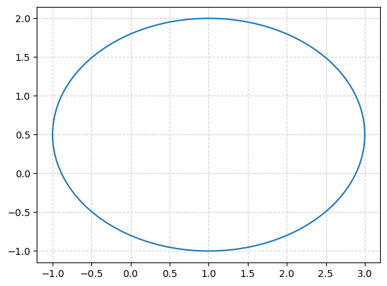
Let us remind ourselves about what an ellipse is before we proceed.
%matplotlib inline

import numpy as np
from matplotlib import pyplot as plt
from math import pi

u=1.     #x-position of the center
v=0.5    #y-position of the center
a=2.     #radius on the x-axis
b=1.5    #radius on the y-axis

t = np.linspace(0, 2*pi, 100)
plt.plot( u+a*np.cos(t) , v+b*np.sin(t) )
plt.grid(color='lightgray',linestyle='--')
plt.show()
6.4. Effective or Centrifugal Potential
The total energy of a particle is
The second term then contributes to the energy like an additional repulsive potential. The term is sometimes referred to as the “centrifugal” potential, even though it is actually the kinetic energy of the angular motion. Combined with \(V(r)\), it is sometimes referred to as the “effective” potential,
Note that if one treats the effective potential like a real potential, one would expect to be able to generate an effective force,
which is indeed matches the form for \(m\ddot{r}\) in Eq. (3), which included the centrifugal force.
The following code plots this effective potential for a simple choice of parameters, with a standard gravitational potential \(-\alpha/r\). Here we have chosen \(L=m=\alpha=1\).
# Common imports
import numpy as np
from math import *
import matplotlib.pyplot as plt

Deltax = 0.01
#set up arrays
xinitial = 0.3
xfinal = 5.0
alpha = 1.0   # spring constant
m = 1.0   # mass, you can change these
AngMom = 1.0  #  The angular momentum
n = ceil((xfinal-xinitial)/Deltax)
x = np.zeros(n)
for i in range(n):
    x[i] = xinitial+i*Deltax
V = np.zeros(n)
V = -alpha/x+0.5*AngMom*AngMom/(m*x*x)
# Plot potential
fig, ax = plt.subplots()
ax.set_xlabel('r[m]')
ax.set_ylabel('V[J]')
ax.plot(x, V)
fig.tight_layout()
plt.show()

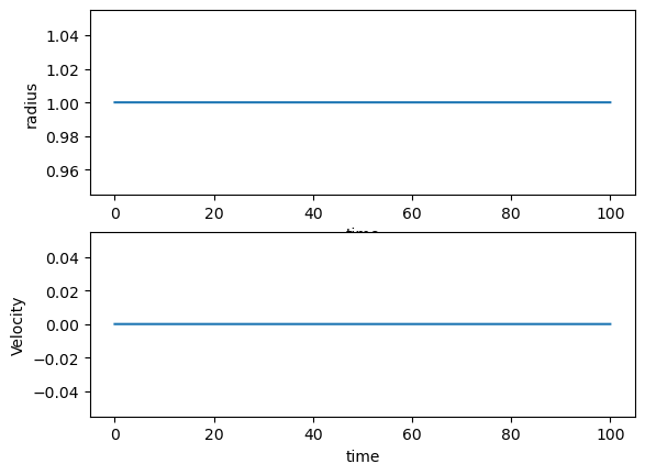
6.4.1. Gravitational force example
Using the above parameters, we can now study the evolution of the system using for example the velocity Verlet method. This is done in the code here for an initial radius equal to the minimum of the potential well. We seen then that the radius is always the same and corresponds to a circle (the radius is always constant).
# Common imports
import numpy as np
import pandas as pd
from math import *
import matplotlib.pyplot as plt
import os

# Where to save the figures and data files
PROJECT_ROOT_DIR = "Results"
FIGURE_ID = "Results/FigureFiles"
DATA_ID = "DataFiles/"

if not os.path.exists(PROJECT_ROOT_DIR):
    os.mkdir(PROJECT_ROOT_DIR)

if not os.path.exists(FIGURE_ID):
    os.makedirs(FIGURE_ID)

if not os.path.exists(DATA_ID):
    os.makedirs(DATA_ID)

def image_path(fig_id):
    return os.path.join(FIGURE_ID, fig_id)

def data_path(dat_id):
    return os.path.join(DATA_ID, dat_id)

def save_fig(fig_id):
    plt.savefig(image_path(fig_id) + ".png", format='png')


# Simple Gravitational Force   -alpha/r

DeltaT = 0.01
#set up arrays
tfinal = 100.0
n = ceil(tfinal/DeltaT)
# set up arrays for t, v and r
t = np.zeros(n)
v = np.zeros(n)
r = np.zeros(n)
# Constants of the model, setting all variables to one for simplicity
alpha = 1.0
AngMom = 1.0  #  The angular momentum
m = 1.0  # scale mass to one
c1 = AngMom*AngMom/(m*m)
c2 = AngMom*AngMom/m
rmin = (AngMom*AngMom/m/alpha)
# Initial conditions
r0 = rmin
v0 = 0.0
r[0] = r0
v[0] = v0
# Start integrating using the Velocity-Verlet  method
for i in range(n-1):
    # Set up acceleration
    a = -alpha/(r[i]**2)+c1/(r[i]**3)
    # update velocity, time and position using the Velocity-Verlet method
    r[i+1] = r[i] + DeltaT*v[i]+0.5*(DeltaT**2)*a
    anew = -alpha/(r[i+1]**2)+c1/(r[i+1]**3)
    v[i+1] = v[i] + 0.5*DeltaT*(a+anew)
    t[i+1] = t[i] + DeltaT
    # Plot position as function of time
fig, ax = plt.subplots(2,1)
ax[0].set_xlabel('time')
ax[0].set_ylabel('radius')
ax[0].plot(t,r)
ax[1].set_xlabel('time')
ax[1].set_ylabel('Velocity')
ax[1].plot(t,v)
save_fig("RadialGVV")
plt.show()
Changing the value of the initial position to a value where the energy is positive, leads to an increasing radius with time, a so-called unbound orbit. Choosing on the other hand an initial radius that corresponds to a negative energy and different from the minimum value leads to a radius that oscillates back and forth between two values.
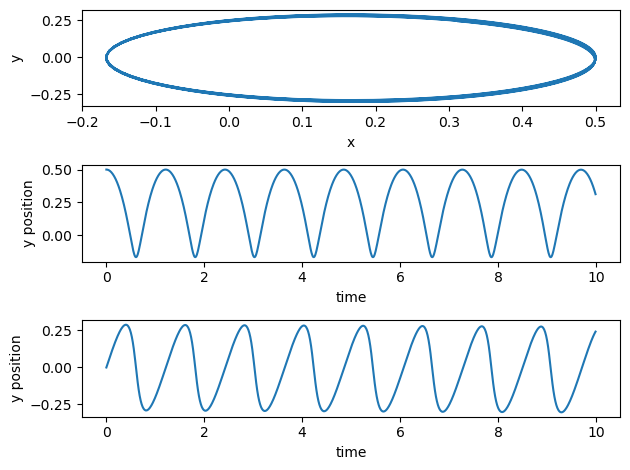
6.4.2. Harmonic Oscillator in two dimensions
Consider a particle of mass \(m\) in a 2-dimensional harmonic oscillator with potential
If the orbit has angular momentum \(L\), we can find the radius and angular velocity of the circular orbit as well as the b) the angular frequency of small radial perturbations.
We consider the effective potential. The radius of a circular orbit is at the minimum of the potential (where the effective force is zero). The potential is plotted here with the parameters \(k=m=0.1\) and \(L=1.0\).
# Common imports
import numpy as np
from math import *
import matplotlib.pyplot as plt

Deltax = 0.01
#set up arrays
xinitial = 0.5
xfinal = 3.0
k = 1.0   # spring constant
m = 1.0   # mass, you can change these
AngMom = 1.0  #  The angular momentum
n = ceil((xfinal-xinitial)/Deltax)
x = np.zeros(n)
for i in range(n):
    x[i] = xinitial+i*Deltax
V = np.zeros(n)
V = 0.5*k*x*x+0.5*AngMom*AngMom/(m*x*x)
# Plot potential
fig, ax = plt.subplots()
ax.set_xlabel('r[m]')
ax.set_ylabel('V[J]')
ax.plot(x, V)
fig.tight_layout()
plt.show()

The effective potential looks like that of a harmonic oscillator for large \(r\), but for small \(r\), the centrifugal potential repels the particle from the origin. The combination of the two potentials has a minimum for at some radius \(r_{\rm min}\).
For particles at \(r_{\rm min}\) with \(\dot{r}=0\), the particle does not accelerate and \(r\) stays constant, i.e. a circular orbit. The radius of the circular orbit can be adjusted by changing the angular momentum \(L\).
For the above parameters this minimum is at \(r_{\rm min}=1\).
Now consider small vibrations about \(r_{\rm min}\). The effective spring constant is the curvature of the effective potential.
Here, the second step used the result of the last step from part (a). Because the radius oscillates with twice the angular frequency, the orbit has two places where \(r\) reaches a minimum in one cycle. This differs from the inverse-square force where there is one minimum in an orbit. One can show that the orbit for the harmonic oscillator is also elliptical, but in this case the center of the potential is at the center of the ellipse, not at one of the foci.
The solution is also simple to write down exactly in Cartesian coordinates. The \(x\) and \(y\) equations of motion separate,
So the general solution can be expressed as
The code here finds the solution for \(x\) and \(y\) using the code we developed in homework 5 and 6 and the midterm. Note that this code is tailored to run in Cartesian coordinates. There is thus no angular momentum dependent term.
DeltaT = 0.01
#set up arrays
tfinal = 10.0
n = ceil(tfinal/DeltaT)
# set up arrays
t = np.zeros(n)
v = np.zeros((n,2))
r = np.zeros((n,2))
radius = np.zeros(n)
# Constants of the model
k = 1.0   # spring constant
m = 1.0   # mass, you can change these
omega02 = sqrt(k/m)  # Frequency
AngMom = 1.0  #  The angular momentum
rmin = (AngMom*AngMom/k/m)**0.25
# Initial conditions as compact 2-dimensional arrays
x0 = rmin-0.5; y0= sqrt(rmin*rmin-x0*x0)
r0 = np.array([x0,y0])
v0 = np.array([0.0,0.0])
r[0] = r0
v[0] = v0
# Start integrating using the Velocity-Verlet  method
for i in range(n-1):
    # Set up the acceleration
    a =  -r[i]*omega02
    # update velocity, time and position using the Velocity-Verlet method
    r[i+1] = r[i] + DeltaT*v[i]+0.5*(DeltaT**2)*a
    anew = -r[i+1]*omega02
    v[i+1] = v[i] + 0.5*DeltaT*(a+anew)
    t[i+1] = t[i] + DeltaT
# Plot position as function of time
radius = np.sqrt(r[:,0]**2+r[:,1]**2)
fig, ax = plt.subplots(3,1)
ax[0].set_xlabel('time')
ax[0].set_ylabel('radius squared')
ax[0].plot(t,r[:,0]**2+r[:,1]**2)
ax[1].set_xlabel('time')
ax[1].set_ylabel('x position')
ax[1].plot(t,r[:,0])
ax[2].set_xlabel('time')
ax[2].set_ylabel('y position')
ax[2].plot(t,r[:,1])

fig.tight_layout()
save_fig("2DimHOVV")
plt.show()
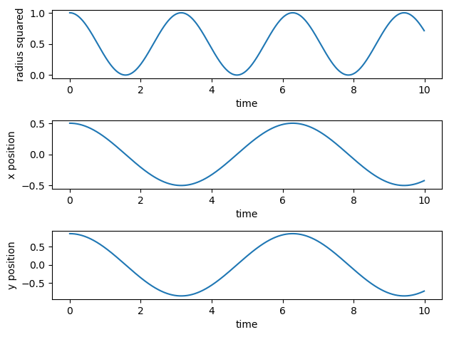
With some work using double angle formulas, one can calculate
and see that radius oscillates with frequency \(2\omega_0\). The factor of two comes because the oscillation \(x=A\cos\omega_0t\) has two maxima for \(x^2\), one at \(t=0\) and one a half period later.
The following code shows first how we can solve this problem using the radial degrees of freedom only.
DeltaT = 0.01
#set up arrays
tfinal = 10.0
n = ceil(tfinal/DeltaT)
# set up arrays for t, v and r
t = np.zeros(n)
v = np.zeros(n)
r = np.zeros(n)
E = np.zeros(n)
# Constants of the model
AngMom = 1.0  #  The angular momentum
m = 1.0
k = 1.0
omega02 = k/m
c1 = AngMom*AngMom/(m*m)
c2 = AngMom*AngMom/m
rmin = (AngMom*AngMom/k/m)**0.25
# Initial conditions
r0 = rmin
v0 = 0.0
r[0] = r0
v[0] = v0
E[0] = 0.5*m*v0*v0+0.5*k*r0*r0+0.5*c2/(r0*r0)
# Start integrating using the Velocity-Verlet  method
for i in range(n-1):
    # Set up acceleration
    a = -r[i]*omega02+c1/(r[i]**3)
    # update velocity, time and position using the Velocity-Verlet method
    r[i+1] = r[i] + DeltaT*v[i]+0.5*(DeltaT**2)*a
    anew = -r[i+1]*omega02+c1/(r[i+1]**3)
    v[i+1] = v[i] + 0.5*DeltaT*(a+anew)
    t[i+1] = t[i] + DeltaT
    E[i+1] = 0.5*m*v[i+1]*v[i+1]+0.5*k*r[i+1]*r[i+1]+0.5*c2/(r[i+1]*r[i+1])
    # Plot position as function of time
fig, ax = plt.subplots(2,1)
ax[0].set_xlabel('time')
ax[0].set_ylabel('radius')
ax[0].plot(t,r)
ax[1].set_xlabel('time')
ax[1].set_ylabel('Energy')
ax[1].plot(t,E)
save_fig("RadialHOVV")
plt.show()

6.5. Stability of Orbits
The effective force can be extracted from the effective potential, \(V_{\rm eff}\). Beginning from the equations of motion, Eq. (1), for \(r\),
For a circular orbit, the radius must be fixed as a function of time, so one must be at a maximum or a minimum of the effective potential. However, if one is at a maximum of the effective potential the radius will be unstable. For the attractive Coulomb force the effective potential will be dominated by the \(-\alpha/r\) term for large \(r\) because the centrifugal part falls off more quickly, \(\sim 1/r^2\). At low \(r\) the centrifugal piece wins and the effective potential is repulsive. Thus, the potential must have a minimum somewhere with negative potential. The circular orbits are then stable to perturbation.
The effective potential is sketched for two cases, a \(1/r\) attractive potential and a \(1/r^3\) attractive potential. The \(1/r\) case has a stable minimum, whereas the circular orbit in the \(1/r^3\) case is unstable.
If one considers a potential that falls as \(1/r^3\), the situation is reversed and the point where \(\partial_rV\) disappears will be a local maximum rather than a local minimum. Fig to come here with code
The repulsive centrifugal piece dominates at large \(r\) and the attractive Coulomb piece wins out at small \(r\). The circular orbit is then at a maximum of the effective potential and the orbits are unstable. It is the clear that for potentials that fall as \(r^n\), that one must have \(n>-2\) for the orbits to be stable.
Consider a potential \(V(r)=\beta r\). For a particle of mass \(m\) with angular momentum \(L\), find the angular frequency of a circular orbit. Then find the angular frequency for small radial perturbations.
For the circular orbit you search for the position \(r_{\rm min}\) where the effective potential is minimized,
Now, we can find the angular frequency of small perturbations about the circular orbit. To do this we find the effective spring constant for the effective potential,
If the two frequencies, \(\dot{\phi}\) and \(\omega\), differ by an integer factor, the orbit’s trajectory will repeat itself each time around. This is the case for the inverse-square force, \(\omega=\dot{\phi}\), and for the harmonic oscillator, \(\omega=2\dot{\phi}\). In this case, \(\omega=\sqrt{3}\dot{\phi}\), and the angles at which the maxima and minima occur change with each orbit.
6.5.1. Code example with gravitional force
The code example here is meant to illustrate how we can make a plot of the final orbit. We solve the equations in polar coordinates (the example here uses the minimum of the potential as initial value) and then we transform back to cartesian coordinates and plot \(x\) versus \(y\). We see that we get a perfect circle when we place ourselves at the minimum of the potential energy, as expected.
# Simple Gravitational Force   -alpha/r

DeltaT = 0.01
#set up arrays
tfinal = 8.0
n = ceil(tfinal/DeltaT)
# set up arrays for t, v and r
t = np.zeros(n)
v = np.zeros(n)
r = np.zeros(n)
phi = np.zeros(n)
x = np.zeros(n)
y = np.zeros(n)
# Constants of the model, setting all variables to one for simplicity
alpha = 1.0
AngMom = 1.0  #  The angular momentum
m = 1.0  # scale mass to one
c1 = AngMom*AngMom/(m*m)
c2 = AngMom*AngMom/m
rmin = (AngMom*AngMom/m/alpha)
# Initial conditions, place yourself at the potential min
r0 = rmin
v0 = 0.0  # starts at rest
r[0] = r0
v[0] = v0
phi[0] = 0.0
# Start integrating using the Velocity-Verlet  method
for i in range(n-1):
    # Set up acceleration
    a = -alpha/(r[i]**2)+c1/(r[i]**3)
    # update velocity, time and position using the Velocity-Verlet method
    r[i+1] = r[i] + DeltaT*v[i]+0.5*(DeltaT**2)*a
    anew = -alpha/(r[i+1]**2)+c1/(r[i+1]**3)
    v[i+1] = v[i] + 0.5*DeltaT*(a+anew)
    t[i+1] = t[i] + DeltaT
    phi[i+1] = t[i+1]*c2/(r0**2)
# Find cartesian coordinates for easy plot
x = r*np.cos(phi)
y = r*np.sin(phi)
fig, ax = plt.subplots(3,1)
ax[0].set_xlabel('time')
ax[0].set_ylabel('radius')
ax[0].plot(t,r)
ax[1].set_xlabel('time')
ax[1].set_ylabel('Angle $\cos{\phi}$')
ax[1].plot(t,np.cos(phi))
ax[2].set_ylabel('y')
ax[2].set_xlabel('x')
ax[2].plot(x,y)

save_fig("Phasespace")
plt.show()
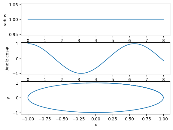
Try to change the initial value for \(r\) and see what kind of orbits you get. In order to test different energies, it can be useful to look at the plot of the effective potential discussed above.
However, for orbits different from a circle the above code would need modifications in order to allow us to display say an ellipse. For the latter, it is much easier to run our code in cartesian coordinates, as done here. In this code we test also energy conservation and see that it is conserved to numerical precision. The code here is a simple extension of the code we developed for homework 4.
# Common imports
import numpy as np
import pandas as pd
from math import *
import matplotlib.pyplot as plt

DeltaT = 0.01
#set up arrays
tfinal = 10.0
n = ceil(tfinal/DeltaT)
# set up arrays
t = np.zeros(n)
v = np.zeros((n,2))
r = np.zeros((n,2))
E = np.zeros(n)
# Constants of the model
m = 1.0   # mass, you can change these
alpha = 1.0
# Initial conditions as compact 2-dimensional arrays
x0 = 0.5; y0= 0.
r0 = np.array([x0,y0])
v0 = np.array([0.0,1.0])
r[0] = r0
v[0] = v0
rabs = sqrt(sum(r[0]*r[0]))
E[0] = 0.5*m*(v[0,0]**2+v[0,1]**2)-alpha/rabs
# Start integrating using the Velocity-Verlet  method
for i in range(n-1):
    # Set up the acceleration
    rabs = sqrt(sum(r[i]*r[i]))
    a =  -alpha*r[i]/(rabs**3)
    # update velocity, time and position using the Velocity-Verlet method
    r[i+1] = r[i] + DeltaT*v[i]+0.5*(DeltaT**2)*a
    rabs = sqrt(sum(r[i+1]*r[i+1]))
    anew = -alpha*r[i+1]/(rabs**3)
    v[i+1] = v[i] + 0.5*DeltaT*(a+anew)
    E[i+1] = 0.5*m*(v[i+1,0]**2+v[i+1,1]**2)-alpha/rabs
    t[i+1] = t[i] + DeltaT
# Plot position as function of time
fig, ax = plt.subplots(3,1)
ax[0].set_ylabel('y')
ax[0].set_xlabel('x')
ax[0].plot(r[:,0],r[:,1])
ax[1].set_xlabel('time')
ax[1].set_ylabel('y position')
ax[1].plot(t,r[:,0])
ax[2].set_xlabel('time')
ax[2].set_ylabel('y position')
ax[2].plot(t,r[:,1])

fig.tight_layout()
save_fig("2DimGravity")
plt.show()
print(E)
[-1.5        -1.49999996 -1.49999984 -1.49999964 -1.49999935 -1.49999898
 -1.49999853 -1.49999798 -1.49999734 -1.49999659 -1.49999574 -1.49999478
 -1.49999369 -1.49999247 -1.49999112 -1.49998961 -1.49998794 -1.49998609
 -1.49998404 -1.49998178 -1.49997929 -1.49997654 -1.49997351 -1.49997017
 -1.49996649 -1.49996243 -1.49995796 -1.49995304 -1.49994762 -1.49994165
 -1.49993508 -1.49992786 -1.49991994 -1.49991127 -1.4999018  -1.49989151
 -1.49988041 -1.49986852 -1.49985595 -1.49984292 -1.49982978 -1.49981712
 -1.49980588 -1.49979754 -1.49979431 -1.49979958 -1.4998184  -1.4998583
 -1.49993028 -1.50005034 -1.50024115 -1.500534   -1.50097003 -1.50159939
 -1.50247522 -1.50363822 -1.5050881  -1.50674417 -1.50841251 -1.50979454
 -1.51056842 -1.5105255  -1.50967788 -1.5082518  -1.50657253 -1.50493047
 -1.50350752 -1.50237442 -1.50152565 -1.50091821 -1.50049876 -1.50021789
 -1.50003547 -1.49992116 -1.49985304 -1.4998157  -1.49979853 -1.49979431
 -1.49979819 -1.49980692 -1.49981835 -1.49983109 -1.49984425 -1.49985725
 -1.49986975 -1.49988156 -1.49989259 -1.49990279 -1.49991218 -1.49992077
 -1.49992862 -1.49993577 -1.49994227 -1.49994819 -1.49995356 -1.49995843
 -1.49996286 -1.49996688 -1.49997052 -1.49997383 -1.49997683 -1.49997955
 -1.49998202 -1.49998426 -1.49998628 -1.49998812 -1.49998977 -1.49999126
 -1.4999926  -1.49999381 -1.49999488 -1.49999583 -1.49999667 -1.49999741
 -1.49999804 -1.49999858 -1.49999903 -1.49999939 -1.49999966 -1.49999986
 -1.49999997 -1.5        -1.49999995 -1.49999982 -1.49999961 -1.49999932
 -1.49999894 -1.49999848 -1.49999792 -1.49999727 -1.49999651 -1.49999565
 -1.49999467 -1.49999357 -1.49999234 -1.49999097 -1.49998945 -1.49998776
 -1.49998589 -1.49998382 -1.49998154 -1.49997902 -1.49997625 -1.49997319
 -1.49996981 -1.4999661  -1.499962   -1.49995749 -1.49995252 -1.49994704
 -1.49994101 -1.49993438 -1.49992709 -1.4999191  -1.49991035 -1.4999008
 -1.49989043 -1.49987924 -1.49986728 -1.49985466 -1.49984159 -1.49982847
 -1.4998159  -1.49980488 -1.49979693 -1.49979438 -1.49980076 -1.49982132
 -1.49986388 -1.49993989 -1.50006592 -1.50026544 -1.50057068 -1.5010238
 -1.50167564 -1.50257898 -1.50377191 -1.50524791 -1.50691602 -1.50857033
 -1.50990493 -1.51060284 -1.51047421 -1.50955526 -1.50808857 -1.50640137
 -1.50477517 -1.50337982 -1.50227653 -1.50145437 -1.5008683  -1.50046492
 -1.50019563 -1.50002129 -1.49991251 -1.49984809 -1.4998132  -1.49979762
 -1.4997944  -1.49979889 -1.49980797 -1.49981959 -1.49983241 -1.49984557
 -1.49985853 -1.49987097 -1.49988271 -1.49989365 -1.49990377 -1.49991308
 -1.49992159 -1.49992937 -1.49993645 -1.4999429  -1.49994875 -1.49995407
 -1.4999589  -1.49996328 -1.49996726 -1.49997087 -1.49997414 -1.49997712
 -1.49997981 -1.49998226 -1.49998447 -1.49998648 -1.49998829 -1.49998993
 -1.4999914  -1.49999273 -1.49999392 -1.49999498 -1.49999592 -1.49999675
 -1.49999747 -1.4999981  -1.49999863 -1.49999907 -1.49999942 -1.49999969
 -1.49999987 -1.49999997 -1.5        -1.49999994 -1.49999981 -1.49999959
 -1.49999929 -1.4999989  -1.49999842 -1.49999786 -1.49999719 -1.49999643
 -1.49999556 -1.49999457 -1.49999346 -1.49999221 -1.49999083 -1.49998929
 -1.49998758 -1.49998569 -1.4999836  -1.4999813  -1.49997876 -1.49997595
 -1.49997286 -1.49996946 -1.4999657  -1.49996157 -1.49995701 -1.49995199
 -1.49994646 -1.49994037 -1.49993368 -1.49992632 -1.49991825 -1.49990942
 -1.49989979 -1.49988934 -1.49987807 -1.49986604 -1.49985336 -1.49984027
 -1.49982716 -1.4998147  -1.49980391 -1.49979638 -1.49979455 -1.49980208
 -1.49982445 -1.49986979 -1.49994999 -1.50008223 -1.50029079 -1.50060886
 -1.50107959 -1.50175446 -1.50268571 -1.50390854 -1.50540978 -1.50708783
 -1.50872493 -1.51000875 -1.51062866 -1.51041471 -1.509427   -1.50792313
 -1.50623094 -1.50462231 -1.50325515 -1.50218152 -1.5013855  -1.50082025
 -1.50043244 -1.50017432 -1.50000777 -1.4999043  -1.49984344 -1.49981089
 -1.49979682 -1.49979457 -1.49979964 -1.49980906 -1.49982085 -1.49983373
 -1.49984689 -1.49985981 -1.49987219 -1.49988385 -1.49989471 -1.49990475
 -1.49991397 -1.49992241 -1.49993011 -1.49993713 -1.49994351 -1.49994931
 -1.49995458 -1.49995936 -1.4999637  -1.49996764 -1.49997121 -1.49997446
 -1.4999774  -1.49998007 -1.49998249 -1.49998468 -1.49998667 -1.49998846
 -1.49999008 -1.49999154 -1.49999286 -1.49999403 -1.49999508 -1.49999601
 -1.49999683 -1.49999754 -1.49999816 -1.49999868 -1.49999911 -1.49999945
 -1.49999971 -1.49999988 -1.49999998 -1.5        -1.49999993 -1.49999979
 -1.49999956 -1.49999925 -1.49999886 -1.49999837 -1.4999978  -1.49999712
 -1.49999635 -1.49999546 -1.49999446 -1.49999334 -1.49999208 -1.49999068
 -1.49998912 -1.4999874  -1.49998549 -1.49998338 -1.49998105 -1.49997849
 -1.49997566 -1.49997253 -1.49996909 -1.4999653  -1.49996113 -1.49995652
 -1.49995145 -1.49994587 -1.49993973 -1.49993297 -1.49992554 -1.4999174
 -1.49990849 -1.49989878 -1.49988824 -1.49987689 -1.49986478 -1.49985205
 -1.49983894 -1.49982587 -1.49981352 -1.49980297 -1.49979589 -1.49979481
 -1.49980355 -1.49982782 -1.49987606 -1.49996062 -1.50009932 -1.50031724
 -1.50064858 -1.50113745 -1.50183589 -1.50279545 -1.50404807 -1.50557355
 -1.50725931 -1.50887594 -1.51010569 -1.51064581 -1.51034718 -1.50929344
 -1.50775585 -1.50606146 -1.504472   -1.50313352 -1.50208936 -1.50131897
 -1.50077398 -1.50040126 -1.50015393 -1.49999488 -1.49989651 -1.49983907
 -1.49980877 -1.49979615 -1.49979481 -1.49980043 -1.49981016 -1.49982211
 -1.49983506 -1.49984821 -1.49986109 -1.4998734  -1.49988498 -1.49989576
 -1.49990571 -1.49991486 -1.49992322 -1.49993085 -1.4999378  -1.49994412
 -1.49994987 -1.49995508 -1.49995982 -1.49996411 -1.49996802 -1.49997156
 -1.49997477 -1.49997768 -1.49998032 -1.49998272 -1.49998489 -1.49998686
 -1.49998863 -1.49999024 -1.49999168 -1.49999298 -1.49999414 -1.49999518
 -1.4999961  -1.4999969  -1.49999761 -1.49999821 -1.49999872 -1.49999914
 -1.49999948 -1.49999973 -1.4999999  -1.49999999 -1.49999999 -1.49999992
 -1.49999977 -1.49999953 -1.49999922 -1.49999881 -1.49999832 -1.49999773
 -1.49999705 -1.49999626 -1.49999537 -1.49999435 -1.49999322 -1.49999195
 -1.49999053 -1.49998896 -1.49998722 -1.49998529 -1.49998316 -1.49998081
 -1.49997821 -1.49997535 -1.4999722  -1.49996873 -1.4999649  -1.49996068
 -1.49995603 -1.49995092 -1.49994528 -1.49993907 -1.49993225 -1.49992475
 -1.49991654 -1.49990755 -1.49989775 -1.49988713 -1.4998757  -1.49986353
 -1.49985074 -1.49983761 -1.49982457 -1.49981235 -1.49980207 -1.49979546
 -1.49979517 -1.49980518 -1.49983142 -1.49988269 -1.49997179 -1.5001172
 -1.50034484 -1.50068989 -1.50119744 -1.50191999 -1.5029082  -1.50419046
 -1.50573905 -1.50743018 -1.50902301 -1.5101955  -1.51065423 -1.51027181
 -1.50915493 -1.50758703 -1.50589314 -1.50432432 -1.50301493 -1.502
 -1.50125473 -1.50072947 -1.50037135 -1.50013443 -1.4999826  -1.49988914
 -1.49983497 -1.49980682 -1.49979559 -1.49979512 -1.49980126 -1.49981129
 -1.49982339 -1.49983638 -1.49984953 -1.49986236 -1.4998746  -1.49988611
 -1.4998968  -1.49990667 -1.49991573 -1.49992402 -1.49993158 -1.49993847
 -1.49994473 -1.49995041 -1.49995558 -1.49996027 -1.49996453 -1.49996839
 -1.49997189 -1.49997507 -1.49997796 -1.49998058 -1.49998295 -1.4999851
 -1.49998704 -1.4999888  -1.49999039 -1.49999182 -1.4999931  -1.49999425
 -1.49999528 -1.49999618 -1.49999698 -1.49999767 -1.49999827 -1.49999877
 -1.49999918 -1.49999951 -1.49999975 -1.49999991 -1.49999999 -1.49999999
 -1.49999991 -1.49999975 -1.49999951 -1.49999918 -1.49999877 -1.49999826
 -1.49999767 -1.49999697 -1.49999618 -1.49999527 -1.49999424 -1.49999309
 -1.49999181 -1.49999038 -1.49998879 -1.49998703 -1.49998508 -1.49998293
 -1.49998056 -1.49997794 -1.49997505 -1.49997187 -1.49996836 -1.49996449
 -1.49996023 -1.49995554 -1.49995037 -1.49994468 -1.49993841 -1.49993153
 -1.49992396 -1.49991567 -1.4999066  -1.49989672 -1.49988602 -1.49987451
 -1.49986226 -1.49984943 -1.49983628 -1.49982329 -1.4998112  -1.4998012
 -1.49979509 -1.49979563 -1.49980697 -1.49983528 -1.49988969 -1.49998353
 -1.50013591 -1.50037362 -1.50073284 -1.50125961 -1.5020068  -1.50302398
 -1.50433563 -1.5059061  -1.50760012 -1.50916579 -1.5102779  -1.51065389
 -1.51018882 -1.5090118  -1.50741701 -1.5057262  -1.50417936 -1.50289938
 -1.5019134  -1.50119273 -1.50068664 -1.50034266 -1.50011579 -1.49997091
 -1.49988216 -1.49983114 -1.49980505 -1.49979514 -1.49979549 -1.49980214
 -1.49981244 -1.49982467 -1.49983771 -1.49985084 -1.49986362 -1.4998758
 -1.49988722 -1.49989783 -1.49990762 -1.4999166  -1.49992482 -1.49993231
 -1.49993912 -1.49994532 -1.49995096 -1.49995607 -1.49996072 -1.49996493
 -1.49996876 -1.49997223 -1.49997538 -1.49997824 -1.49998083 -1.49998318
 -1.4999853  -1.49998723 -1.49998897 -1.49999054 -1.49999196 -1.49999323
 -1.49999436 -1.49999537 -1.49999627 -1.49999705 -1.49999774 -1.49999832
 -1.49999881 -1.49999922 -1.49999954 -1.49999977 -1.49999992 -1.49999999
 -1.49999999 -1.4999999  -1.49999973 -1.49999948 -1.49999914 -1.49999872
 -1.49999821 -1.4999976  -1.4999969  -1.49999609 -1.49999517 -1.49999413
 -1.49999297 -1.49999167 -1.49999023 -1.49998862 -1.49998684 -1.49998488
 -1.4999827  -1.4999803  -1.49997766 -1.49997474 -1.49997153 -1.49996799
 -1.49996408 -1.49995978 -1.49995504 -1.49994982 -1.49994408 -1.49993775
 -1.49993079 -1.49992316 -1.49991479 -1.49990564 -1.49989568 -1.49988489
 -1.49987331 -1.49986099 -1.49984811 -1.49983496 -1.49982202 -1.49981008
 -1.49980037 -1.49979479 -1.4997962  -1.49980893 -1.4998394  -1.4998971
 -1.49999586 -1.50015547 -1.50040363 -1.5007775  -1.50132402 -1.50209638
 -1.50314281 -1.50448352 -1.50607451 -1.50776883 -1.50930394 -1.51035268
 -1.5106448  -1.51009845 -1.50886441 -1.50724608 -1.50556083 -1.50403719
 -1.50278686 -1.50182951 -1.50113291 -1.50064545 -1.50031516 -1.50009797
 -1.49995978 -1.49987556 -1.49982755 -1.49980343 -1.49979479 -1.49979593
 -1.49980304 -1.49981361 -1.49982597 -1.49983904 -1.49985215 -1.49986488
 -1.49987698 -1.49988833 -1.49989886 -1.49990856 -1.49991746 -1.4999256
 -1.49993302 -1.49993978 -1.49994592 -1.4999515  -1.49995656 -1.49996116
 -1.49996533 -1.49996912 -1.49997256 -1.49997568 -1.49997851 -1.49998107
 -1.4999834  -1.49998551 -1.49998741 -1.49998914 -1.49999069 -1.49999209
 -1.49999335 -1.49999447 -1.49999547 -1.49999635 -1.49999713 -1.4999978
 -1.49999838 -1.49999886 -1.49999925 -1.49999956 -1.49999979 -1.49999993
 -1.5        -1.49999998 -1.49999988 -1.49999971 -1.49999945 -1.4999991
 -1.49999867 -1.49999815 -1.49999754 -1.49999682 -1.499996   -1.49999507
 -1.49999402 -1.49999285 -1.49999153 -1.49999007 -1.49998845 -1.49998665
 -1.49998467 -1.49998247 -1.49998005 -1.49997738 -1.49997443 -1.49997119
 -1.49996761 -1.49996367 -1.49995932 -1.49995454 -1.49994927 -1.49994346
 -1.49993708 -1.49993006 -1.49992235 -1.4999139  -1.49990467 -1.49989463
 -1.49988376 -1.4998721  -1.49985972 -1.49984679 -1.49983363 -1.49982075
 -1.49980897 -1.49979958 -1.49979455 -1.49979688 -1.49981106 -1.49984379
 -1.49990491 -1.50000879 -1.50017593 -1.5004349  -1.50082389 -1.50139073
 -1.50218876 -1.50326468 -1.50463403 -1.50624407 -1.50793598 -1.5094371
 -1.5104196  -1.51062698 -1.51000097 -1.50871311 -1.50707457 -1.50539721
 -1.50389788 -1.50267736 -1.50174828 -1.50107521 -1.50060585 -1.50028879
 -1.50008095 -1.49994919 -1.49986932 -1.4998242  -1.49980197 -1.49979453
 -1.49979642 -1.49980398 -1.49981479 -1.49982726 -1.49984037 -1.49985346
 -1.49986613 -1.49987816 -1.49988943 -1.49989987 -1.49990949 -1.49991832
 -1.49992638 -1.49993373 -1.49994042 -1.4999465  -1.49995203 -1.49995705
 -1.4999616  -1.49996573 -1.49996948 -1.49997289 -1.49997598 -1.49997878
 -1.49998132 -1.49998362 -1.49998571 -1.4999876  -1.4999893  -1.49999084
 -1.49999222 -1.49999347 -1.49999458 -1.49999556 -1.49999644 -1.4999972
 -1.49999786 -1.49999843 -1.4999989  -1.49999929 -1.49999959 -1.49999981
 -1.49999994 -1.5        -1.49999997 -1.49999987 -1.49999968 -1.49999942
 -1.49999906 -1.49999862 -1.49999809 -1.49999747 -1.49999674 -1.49999591
 -1.49999497 -1.49999391 -1.49999272 -1.49999139 -1.49998992 -1.49998828
 -1.49998646 -1.49998446 -1.49998224 -1.49997979 -1.49997709 -1.49997412
 -1.49997084 -1.49996723 -1.49996325 -1.49995886 -1.49995403 -1.49994871
 -1.49994285 -1.4999364  -1.49992931 -1.49992153]
6.6. Scattering and Cross Sections
Scattering experiments don’t measure entire trajectories. For elastic collisions, they measure the distribution of final scattering angles at best. Most experiments use targets thin enough so that the number of scatterings is typically zero or one. The cross section, \(\sigma\), describes the cross-sectional area for particles to scatter with an individual target atom or nucleus. Cross section measurements form the basis for MANY fields of physics. BThe cross section, and the differential cross section, encapsulates everything measurable for a collision where all that is measured is the final state, e.g. the outgoing particle had momentum \(\boldsymbol{p}_f\). y studying cross sections, one can infer information about the potential interaction between the two particles. Inferring, or constraining, the potential from the cross section is a classic {\it inverse} problem. Collisions are either elastic or inelastic. Elastic collisions are those for which the two bodies are in the same internal state before and after the collision. If the collision excites one of the participants into a higher state, or transforms the particles into different species, or creates additional particles, the collision is inelastic. Here, we consider only elastic collisions.
For Coulomb forces, the cross section is infinite because the range of the Coulomb force is infinite, but for interactions such as the strong interaction in nuclear or particle physics, there is no long-range force and cross-sections are finite. Even for Coulomb forces, the part of the cross section that corresponds to a specific scattering angle, \(d\sigma/d\Omega\), which is a function of the scattering angle \(\phi_s\) is still finite.
If a particle travels through a thin target, the chance the particle scatters is \(P_{\rm scatt}=\sigma dN/dA\), where \(dN/dA\) is the number of scattering centers per area the particle encounters. If the density of the target is \(\rho\) particles per volume, and if the thickness of the target is \(t\), the areal density (number of target scatterers per area) is \(dN/dA=\rho t\). Because one wishes to quantify the collisions independently of the target, experimentalists measure scattering probabilities, then divide by the areal density to obtain cross-sections,
Instead of merely stating that a particle collided, one can measure the probability the particle scattered by a given angle. The scattering angle \(\phi_s\) is defined so that at zero the particle is unscattered and at \(\phi_s=\pi\) the particle is scattered directly backward. Scattering angles are often described in the center-of-mass frame, but that is a detail we will neglect for this first discussion, where we will consider the scattering of particles moving classically under the influence of fixed potentials \(U(\boldsymbol{r})\). Because the distribution of scattering angles can be measured, one expresses the differential cross section,
Usually, the literature expresses differential cross sections as
where the last equivalency is true when the scattering does not depend on the azimuthal angle \(\phi\), as is the case for spherically symmetric potentials.
The differential solid angle \(d\Omega\) can be thought of as the area subtended by a measurement, \(dA_d\), divided by \(r^2\), where \(r\) is the distance to the detector,
With this definition \(d\sigma/d\Omega\) is independent of the distance from which one places the detector, or the size of the detector (as long as it is small).
Differential scattering cross sections are calculated by assuming a random distribution of impact parameters \(b\). These represent the distance in the \(xy\) plane for particles moving in the \(z\) direction relative to the scattering center. An impact parameter \(b=0\) refers to being aimed directly at the target’s center. The impact parameter describes the transverse distance from the \(z=0\) axis for the trajectory when it is still far away from the scattering center and has not yet passed it. The differential cross section can be expressed in terms of the impact parameter,
which is the area of a thin ring of radius \(b\) and thickness \(db\). In classical physics, one can calculate the trajectory given the incoming kinetic energy \(E\) and the impact parameter if one knows the mass and potential. From the trajectory, one then finds the scattering angle \(\phi_s(b)\). The differential cross section is then
Typically, one would calculate \(\cos\phi_s\) and \((d/db)\cos\phi_s\) as functions of \(b\). This is sufficient to plot the differential cross section as a function of \(\phi_s\).
The total cross section is
Even if the total cross section is infinite, e.g. Coulomb forces, one can still have a finite differential cross section as we will see later on.
An asteroid of mass \(m\) and kinetic energy \(E\) approaches a planet of radius \(R\) and mass \(M\). What is the cross section for the asteroid to impact the planet?
6.6.1. Solution
Calculate the maximum impact parameter, \(b_{\rm max}\), for which the asteroid will hit the planet. The total cross section for impact is \(\sigma_{\rm impact}=\pi b_{\rm max}^2\). The maximum cross-section can be found with the help of angular momentum conservation. The asteroid’s incoming momentum is \(p_0=\sqrt{2mE}\) and the angular momentum is \(L=p_0b\). If the asteroid just grazes the planet, it is moving with zero radial kinetic energy at impact. Combining energy and angular momentum conservation and having \(p_f\) refer to the momentum of the asteroid at a distance \(R\),
allows one to solve for \(b_{\rm max}\),
6.7. Rutherford Scattering
This refers to the calculation of \(d\sigma/d\Omega\) due to an inverse square force, \(F_{12}=\pm\alpha/r^2\) for repulsive/attractive interaction. Rutherford compared the scattering of \(\alpha\) particles (\(^4\)He nuclei) off of a nucleus and found the scattering angle at which the formula began to fail. This corresponded to the impact parameter for which the trajectories would strike the nucleus. This provided the first measure of the size of the atomic nucleus. At the time, the distribution of the positive charge (the protons) was considered to be just as spread out amongst the atomic volume as the electrons. After Rutherford’s experiment, it was clear that the radius of the nucleus tended to be roughly 4 orders of magnitude smaller than that of the atom, which is less than the size of a football relative to Spartan Stadium.
The incoming and outgoing angles of the trajectory are at \(\pm\phi'\). They are related to the scattering angle by \(2\phi'=\pi+\phi_s\).
In order to calculate differential cross section, we must find how the impact parameter is related to the scattering angle. This requires analysis of the trajectory. We consider our previous expression for the trajectory where we derived the elliptic form for the trajectory, Eq. (9). For that case we considered an attractive force with the particle’s energy being negative, i.e. it was bound. However, the same form will work for positive energy, and repulsive forces can be considered by simple flipping the sign of \(\alpha\). For positive energies, the trajectories will be hyperbolas, rather than ellipses, with the asymptotes of the trajectories representing the directions of the incoming and outgoing tracks. Rewriting Eq. (9),
Once \(A\) is large enough, which will happen when the energy is positive, the denominator will become negative for a range of \(\phi\). This is because the scattered particle will never reach certain angles. The asymptotic angles \(\phi'\) are those for which the denominator goes to zero,
The trajectory’s point of closest approach is at \(\phi=0\) and the two angles \(\phi'\), which have this value of \(\cos\phi'\), are the angles of the incoming and outgoing particles. From Fig (to come), one can see that the scattering angle \(\phi_s\) is given by,
Now that we have \(\phi_s\) in terms of \(m,\alpha,L\) and \(A\), we wish to re-express \(L\) and \(A\) in terms of the impact parameter \(b\) and the energy \(E\). This will set us up to calculate the differential cross section, which requires knowing \(db/d\phi_s\). It is easy to write the angular momentum as
Finding \(A\) is more complicated. To accomplish this we realize that the point of closest approach occurs at \(\phi=0\), so from Eq. (15)
Next, \(r_{\rm min}\) can be found in terms of the energy because at the point of closest approach the kinetic energy is due purely to the motion perpendicular to \(\hat{r}\) and
One can solve the quadratic equation for \(1/r_{\rm min}\),
We can plug the expression for \(r_{\rm min}\) into the expression for \(A\), Eq. (19),
Finally, we insert the expression for \(A\) into that for the scattering angle, Eq. (17),
The differential cross section can now be found by differentiating the expression for \(\phi_s\) with \(b\),
where \(a= \alpha/2E\). This the Rutherford formula for the differential cross section. It diverges as \(\phi_s\rightarrow 0\) because scatterings with arbitrarily large impact parameters still scatter to arbitrarily small scattering angles. The expression for \(d\sigma/d\Omega\) is the same whether the interaction is positive or negative.
Consider a particle of mass \(m\) and charge \(z\) with kinetic energy \(E\) (Let it be the center-of-mass energy) incident on a heavy nucleus of mass \(M\) and charge \(Z\) and radius \(R\). Find the angle at which the Rutherford scattering formula breaks down.
6.7.1. Solution
Let \(\alpha=Zze^2/(4\pi\epsilon_0)\). The scattering angle in Eq. (23) is
The impact parameter \(b\) for which the point of closest approach equals \(R\) can be found by using angular momentum conservation,
Putting these together
It was from this departure of the experimentally measured \(d\sigma/d\Omega\) from the Rutherford formula that allowed Rutherford to infer the radius of the gold nucleus, \(R\).
Just like electrodynamics, one can define “fields”, which for a small additional mass \(m\) are the force per mass and the additional potential energy per mass. The {\it gravitational field} related to the force has dimensions of force per mass, or acceleration, and can be labeled \(\boldsymbol{g}(\boldsymbol{r})\). The potential energy per mass has dimensions of energy per mass. This is analogous to the electromagnetic potential, which is the potential energy per charge, and the electric field which is the force per charge.
Because the field \(\boldsymbol{g}\) obeys the same inverse square law for a point mass as the electric field does for a point charge, the gravitational field also satisfies a version of Gauss’s law,
Here, \(M_{\rm inside}\) is the net mass inside a closed area.
Gauss’s law can be understood by considering a nozzle that sprays paint in all directions uniformly from a point source. Let \(B\) be the number of gallons per minute of paint leaving the nozzle. If the nozzle is at the center of a sphere of radius \(r\), the paint per square meter per minute that is deposited on some part of the sphere
Now, let \(F\) also be assigned a direction, so that it becomes a vector pointing along the direction of the flying paint. For any surface that surrounds the nozzle, not necessarily a sphere, one can state that
regardless of the shape of the surface. This follows because the rate at which paint is deposited on the surface should equal the rate at which it leaves the nozzle. The dot product ensures that only the component of \(\boldsymbol{F}\) into the surface contributes to the deposition of paint. Similarly, if \(\boldsymbol{F}\) is any radial inverse-square forces, that falls as \(B/(4\pi r^2)\), then one can apply Eq. (26). For gravitational fields, \(B/(4\pi)\) is replaced by \(GM\), and one quickly “derives” Gauss’s law for gravity, Eq. (25).
Consider Earth to have its mass \(M\) uniformly distributed in a sphere of radius \(R\). Find the magnitude of the gravitational acceleration as a function of the radius \(r\) in terms of the acceleration of gravity at the surface \(g(R)\). Assume \(r<R\), i.e. you are inside the surface.
{\bf Solution}: Take the ratio of Eq. (25) for two radii, \(R\) and \(r<R\),
The potential energy per mass is similar conceptually to the voltage, or electric potential energy per charge, that was studied in electromagnetism, if \(V\equiv U/m\), \(\boldsymbol{g}=-\nabla V\).
6.8. Tidal Forces
Consider a spherical planet of radius \(r\) a distance \(D\) from another body of mass \(M\). The magnitude of the force due to \(M\) on an small object of mass \(\delta m\) on surface of the planet can be calculated by performing a Taylor expansion about the center of the spherical planet.
If the \(z\) direction points toward the large object, \(\Delta D\) can be referred to as \(z\). In the accelerating frame of an observer at the center of the planet,
where \(a'\) is the acceleration of the observer. Because \(\delta ma'\) equals the gravitational force on \(\delta m\) if it were located at the planet’s center, one can write
Here the other forces could represent the forces acting on \(\delta m\) from the spherical planet such as the gravitational force or the contact force with the surface. If \(\phi\) is the angle w.r.t. the \(z\) axis, the effective force acting on \(\delta m\) is
This first force is the “tidal” force. It pulls objects outward from the center of the object. If the object were covered with water, it would distort the objects shape so that the shape would be elliptical, stretched out along the axis pointing toward the large mass \(M\). The force is always along (either parallel or antiparallel to) the \(\hat{z}\) direction.
Consider the Earth to be a sphere of radius \(R\) covered with water, with the gravitational acceleration at the surface noted by \(g\). Now assume that a distant body provides an additional constant gravitational acceleration \(\boldsymbol{a}\) pointed along the \(z\) axis. Find the distortion of the radius as a function of \(\phi\). Ignore planetary rotation and assume \(a<<g\).
{\bf Solution}: Because Earth would then accelerate with \(a\), the field \(a\) would seem invisible in the accelerating frame. A tidal force would only appear if \(a\) depended on position, i.e. \(\nabla \boldsymbol{a}\ne 0\).
Now consider that the field is no longer constant, but that instead \(a=-kz\) with \(|kR|<<g\).
{\bf Solution}: The surface of the planet needs to be at constant potential (if the planet is not accelerating). The force per mass, \(-kz\) is like a spring, and the potential per mass is \(kz^2/2\). Otherwise water would move to a point of lower potential. Thus, the potential energy for a sample mass \(\delta m\) is
Here, the potential due to the external field is \((1/2)kz^2\) so that \(-\nabla U=-kz\). One now needs to solve for \(h(\phi)\). Absorbing all the constant terms from both sides of the equation into one constant \(C\), and because both \(h\) and \(kR\) are small, we can through away terms of order \(h^2\) or \(kRh\). This gives
The term with the factor of \(1/3\) replaced the constant and was chosen so that the average height of the water would be zero.
The Sun’s mass is \(27\times 10^6\) the Moon’s mass, but the Sun is 390 times further away from Earth as the Sun. What is ratio of the tidal force of the Sun to that of the Moon.
{\bf Solution}: The gravitational force due to an object \(M\) a distance \(D\) away goes as \(M/D^2\), but the tidal force is only the difference of that force over a distance \(R\),
Therefore the ratio of force is
The Moon more strongly affects tides than the Sun.
6.9. Exercises
6.9.1. The Earth-Sun System
We start with a simpler case first, the Earth-Sun system in two dimensions only. The gravitational force \(F_G\) on the earth from the sun is
where \(G\) is the gravitational constant,
the mass of Earth,
the mass of the Sun and
is the distance between Earth and the Sun. The latter defines what we call an astronomical unit AU. From Newton’s second law we have then for the \(x\) direction
and
for the \(y\) direction.
Here we will use that \(x=r\cos{(\theta)}\), \(y=r\sin{(\theta)}\) and
We can rewrite these equations
and
as four first-order coupled differential equations
and
and
and
The four coupled differential equations
and
and
and
can be turned into dimensionless equations or we can introduce astronomical units with \(1\) AU = \(1.5\times 10^{11}\).
Using the equations from circular motion (with \(r =1\mathrm{AU}\))
we have
and using that the velocity of Earth (assuming circular motion) is \(v = 2\pi r/\mathrm{yr}=2\pi\mathrm{AU}/\mathrm{yr}\), we have
The four coupled differential equations can then be discretized using Euler’s method as (with step length \(h\))
and
and
and
The code here implements Euler’s method for the Earth-Sun system using a more compact way of representing the vectors. Alternatively, you could have spelled out all the variables \(v_x\), \(v_y\), \(x\) and \(y\) as one-dimensional arrays.
# Common imports
import numpy as np
import pandas as pd
from math import *
import matplotlib.pyplot as plt
import os

# Where to save the figures and data files
PROJECT_ROOT_DIR = "Results"
FIGURE_ID = "Results/FigureFiles"
DATA_ID = "DataFiles/"

if not os.path.exists(PROJECT_ROOT_DIR):
    os.mkdir(PROJECT_ROOT_DIR)

if not os.path.exists(FIGURE_ID):
    os.makedirs(FIGURE_ID)

if not os.path.exists(DATA_ID):
    os.makedirs(DATA_ID)

def image_path(fig_id):
    return os.path.join(FIGURE_ID, fig_id)

def data_path(dat_id):
    return os.path.join(DATA_ID, dat_id)

def save_fig(fig_id):
    plt.savefig(image_path(fig_id) + ".png", format='png')


DeltaT = 0.01
#set up arrays
tfinal = 10 # in years
n = ceil(tfinal/DeltaT)
# set up arrays for t, a, v, and x
t = np.zeros(n)
v = np.zeros((n,2))
r = np.zeros((n,2))
# Initial conditions as compact 2-dimensional arrays
r0 = np.array([1.0,0.0])
v0 = np.array([0.0,2*pi])
r[0] = r0
v[0] = v0
Fourpi2 = 4*pi*pi
# Start integrating using Euler's method
for i in range(n-1):
    # Set up the acceleration
    # Here you could have defined your own function for this
    rabs = sqrt(sum(r[i]*r[i]))
    a =  -Fourpi2*r[i]/(rabs**3)
    # update velocity, time and position using Euler's forward method
    v[i+1] = v[i] + DeltaT*a
    r[i+1] = r[i] + DeltaT*v[i]
    t[i+1] = t[i] + DeltaT
# Plot position as function of time
fig, ax = plt.subplots()
#ax.set_xlim(0, tfinal)
ax.set_xlabel('x[AU]')
ax.set_ylabel('y[AU]')
ax.plot(r[:,0], r[:,1])
fig.tight_layout()
save_fig("EarthSunEuler")
plt.show()
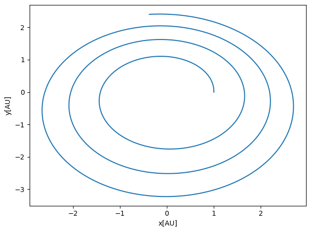
We notice here that Euler’s method doesn’t give a stable orbit with for example \(\Delta t =0.01\). It means that we cannot trust Euler’s method. Euler’s method does not conserve energy. It is an example of an integrator which is not symplectic.
Here we present thus two methods, which with simple changes allow us to avoid these pitfalls. The simplest possible extension is the so-called Euler-Cromer method. The changes we need to make to our code are indeed marginal here. We need simply to replace
r[i+1] = r[i] + DeltaT*v[i]
in the above code with the velocity at the new time \(t_{i+1}\)
r[i+1] = r[i] + DeltaT*v[i+1]
By this simple caveat we get stable orbits. Below we derive the Euler-Cromer method as well as one of the most utlized algorithms for solving the above type of problems, the so-called Velocity-Verlet method.
Let us repeat Euler’s method. We have a differential equation
and if we truncate at the first derivative, we have from the Taylor expansion
which when complemented with \(t_{i+1}=t_i+\Delta t\) forms the algorithm for the well-known Euler method. Note that at every step we make an approximation error of the order of \(O(\Delta t^2)\), however the total error is the sum over all steps \(N=(b-a)/(\Delta t)\) for \(t\in [a,b]\), yielding thus a global error which goes like \(NO(\Delta t^2)\approx O(\Delta t)\).
To make Euler’s method more precise we can obviously decrease \(\Delta t\) (increase \(N\)), but this can lead to loss of numerical precision. Euler’s method is not recommended for precision calculation, although it is handy to use in order to get a first view on how a solution may look like.
Euler’s method is asymmetric in time, since it uses information about the derivative at the beginning of the time interval. This means that we evaluate the position at \(y_1\) using the velocity at \(v_0\). A simple variation is to determine \(x_{n+1}\) using the velocity at \(v_{n+1}\), that is (in a slightly more generalized form)
and
The acceleration \(a_n\) is a function of \(a_n(y_n, v_n, t_n)\) and needs to be evaluated as well. This is the Euler-Cromer method. It is easy to change the above code and see that with the same time step we get stable results.
Let us stay with \(x\) (position) and \(v\) (velocity) as the quantities we are interested in.
We have the Taylor expansion for the position given by
The corresponding expansion for the velocity is
Via Newton’s second law we have normally an analytical expression for the derivative of the velocity, namely
If we add to this the corresponding expansion for the derivative of the velocity
and retain only terms up to the second derivative of the velocity since our error goes as \(O(h^3)\), we have
We can then rewrite the Taylor expansion for the velocity as
Our final equations for the position and the velocity become then
and
Note well that the term \(a_{i+1}\) depends on the position at \(x_{i+1}\). This means that you need to calculate the position at the updated time \(t_{i+1}\) before the computing the next velocity. Note also that the derivative of the velocity at the time \(t_i\) used in the updating of the position can be reused in the calculation of the velocity update as well.
We can now easily add the Verlet method to our original code as
DeltaT = 0.01
#set up arrays
tfinal = 10
n = ceil(tfinal/DeltaT)
# set up arrays for t, a, v, and x
t = np.zeros(n)
v = np.zeros((n,2))
r = np.zeros((n,2))
# Initial conditions as compact 2-dimensional arrays
r0 = np.array([1.0,0.0])
v0 = np.array([0.0,2*pi])
r[0] = r0
v[0] = v0
Fourpi2 = 4*pi*pi
# Start integrating using the Velocity-Verlet  method
for i in range(n-1):
    # Set up forces, air resistance FD, note now that we need the norm of the vecto
    # Here you could have defined your own function for this
    rabs = sqrt(sum(r[i]*r[i]))
    a =  -Fourpi2*r[i]/(rabs**3)
    # update velocity, time and position using the Velocity-Verlet method
    r[i+1] = r[i] + DeltaT*v[i]+0.5*(DeltaT**2)*a
    rabs = sqrt(sum(r[i+1]*r[i+1]))
    anew = -4*(pi**2)*r[i+1]/(rabs**3)
    v[i+1] = v[i] + 0.5*DeltaT*(a+anew)
    t[i+1] = t[i] + DeltaT
# Plot position as function of time
fig, ax = plt.subplots()
ax.set_xlabel('x[AU]')
ax.set_ylabel('y[AU]')
ax.plot(r[:,0], r[:,1])
fig.tight_layout()
save_fig("EarthSunVV")
plt.show()
You can easily generalize the calculation of the forces by defining a function which takes in as input the various variables. We leave this as a challenge to you.
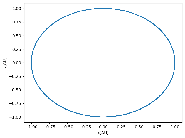
Running the above code for various time steps we see that the Velocity-Verlet is fully stable for various time steps.
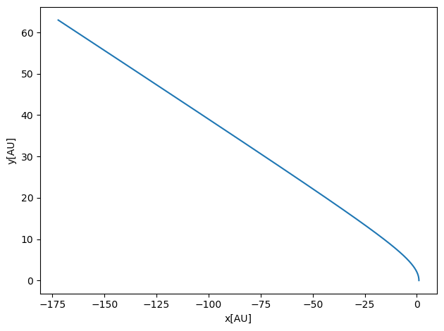
We can also play around with different initial conditions in order to find the escape velocity from an orbit around the sun with distance one astronomical unit, 1 AU. The theoretical value for the escape velocity, is given by
and with \(r=1\) AU, this means that the escape velocity is \(2\pi\sqrt{2}\) AU/yr. To obtain this we required that the kinetic energy of Earth equals the potential energy given by the gravitational force.
Setting
and with \(GM_{\odot}=4\pi^2\) we obtain the above relation for the velocity. Setting an initial velocity say equal to \(9\) in the above code, yields a planet (Earth) which escapes a stable orbit around the sun, as seen by running the code here.
DeltaT = 0.01
#set up arrays
tfinal = 100
n = ceil(tfinal/DeltaT)
# set up arrays for t, a, v, and x
t = np.zeros(n)
v = np.zeros((n,2))
r = np.zeros((n,2))
# Initial conditions as compact 2-dimensional arrays
r0 = np.array([1.0,0.0])
# setting initial velocity larger than escape velocity
v0 = np.array([0.0,9.0])
r[0] = r0
v[0] = v0
Fourpi2 = 4*pi*pi
# Start integrating using the Velocity-Verlet  method
for i in range(n-1):
    # Set up forces, air resistance FD, note now that we need the norm of the vecto
    # Here you could have defined your own function for this
    rabs = sqrt(sum(r[i]*r[i]))
    a =  -Fourpi2*r[i]/(rabs**3)
    # update velocity, time and position using the Velocity-Verlet method
    r[i+1] = r[i] + DeltaT*v[i]+0.5*(DeltaT**2)*a
    rabs = sqrt(sum(r[i+1]*r[i+1]))
    anew = -4*(pi**2)*r[i+1]/(rabs**3)
    v[i+1] = v[i] + 0.5*DeltaT*(a+anew)
    t[i+1] = t[i] + DeltaT
# Plot position as function of time
fig, ax = plt.subplots()
ax.set_xlabel('x[AU]')
ax.set_ylabel('y[AU]')
ax.plot(r[:,0], r[:,1])
fig.tight_layout()
save_fig("EscapeEarthSunVV")
plt.show()
6.9.2. Testing Energy conservation
The code here implements Euler’s method for the Earth-Sun system using a more compact way of representing the vectors. Alternatively, you could have spelled out all the variables \(v_x\), \(v_y\), \(x\) and \(y\) as one-dimensional arrays. It tests conservation of potential and kinetic energy as functions of time, in addition to the total energy, again as function of time
Note: in all codes we have used scaled equations so that the gravitational constant times the mass of the sum is given by \(4\pi^2\) and the mass of the earth is set to one in the calculations of kinetic and potential energies. Else, we would get very large results.
# Common imports
import numpy as np
import pandas as pd
from math import *
import matplotlib.pyplot as plt
import os

# Where to save the figures and data files
PROJECT_ROOT_DIR = "Results"
FIGURE_ID = "Results/FigureFiles"
DATA_ID = "DataFiles/"

if not os.path.exists(PROJECT_ROOT_DIR):
    os.mkdir(PROJECT_ROOT_DIR)

if not os.path.exists(FIGURE_ID):
    os.makedirs(FIGURE_ID)

if not os.path.exists(DATA_ID):
    os.makedirs(DATA_ID)

def image_path(fig_id):
    return os.path.join(FIGURE_ID, fig_id)

def data_path(dat_id):
    return os.path.join(DATA_ID, dat_id)

def save_fig(fig_id):
    plt.savefig(image_path(fig_id) + ".png", format='png')

# Initial values, time step, positions and velocites

DeltaT = 0.0001
#set up arrays
tfinal = 100 # in years
n = ceil(tfinal/DeltaT)
# set up arrays for t, a, v, and x
t = np.zeros(n)
v = np.zeros((n,2))
r = np.zeros((n,2))

# setting up the kinetic, potential and total energy, note only functions of time
EKinetic = np.zeros(n)
EPotential = np.zeros(n)
ETotal = np.zeros(n)

# Initial conditions as compact 2-dimensional arrays


r0 = np.array([1.0,0.0])
v0 = np.array([0.0,2*pi])
r[0] = r0
v[0] = v0
Fourpi2 = 4*pi*pi
# Setting up variables for the calculation of energies
#  distance that defines rabs in potential energy
rabs0 = sqrt(sum(r[0]*r[0]))
#  Initial kinetic energy. Note that we skip the mass of the Earth here, that is MassEarth=1 in all codes
EKinetic[0] = 0.5*sum(v0*v0)
#  Initial potential energy  (note negative sign, why?)
EPotential[0] = -4*pi*pi/rabs0
#  Initial total energy
ETotal[0] = EPotential[0]+EKinetic[0]
# Start integrating using Euler's method
for i in range(n-1):
    # Set up the acceleration
    # Here you could have defined your own function for this
    rabs = sqrt(sum(r[i]*r[i]))
    a =  -Fourpi2*r[i]/(rabs**3)
    # update Energies, velocity, time and position using Euler's forward method
    v[i+1] = v[i] + DeltaT*a
    r[i+1] = r[i] + DeltaT*v[i]
    t[i+1] = t[i] + DeltaT
    EKinetic[i+1] = 0.5*sum(v[i+1]*v[i+1])
    EPotential[i+1] = -4*pi*pi/sqrt(sum(r[i+1]*r[i+1]))
    ETotal[i+1] = EPotential[i+1]+EKinetic[i+1]
# Plot energies as functions of time

fig, axs = plt.subplots(3, 1)
axs[0].plot(t, EKinetic)
axs[0].set_xlim(0, tfinal)
axs[0].set_ylabel('Kinetic energy')
axs[1].plot(t, EPotential)
axs[1].set_ylabel('Potential Energy')
axs[2].plot(t, ETotal)
axs[2].set_xlabel('Time [yr]')
axs[2].set_ylabel('Total Energy')
fig.tight_layout()
save_fig("EarthSunEuler")
plt.show()
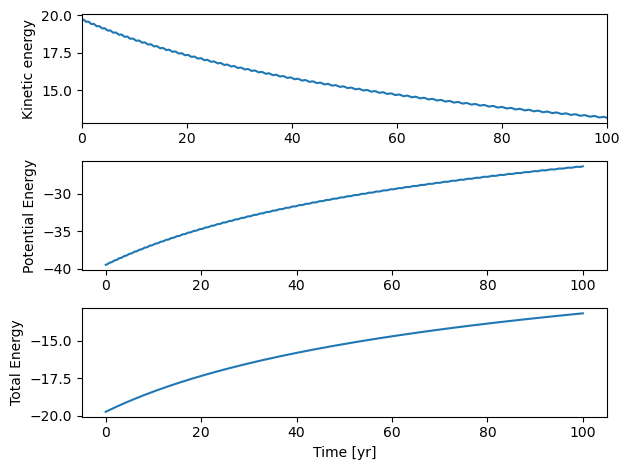
We see very clearly that Euler’s method does not conserve energy!! Try to reduce the time step \(\Delta t\). What do you see?
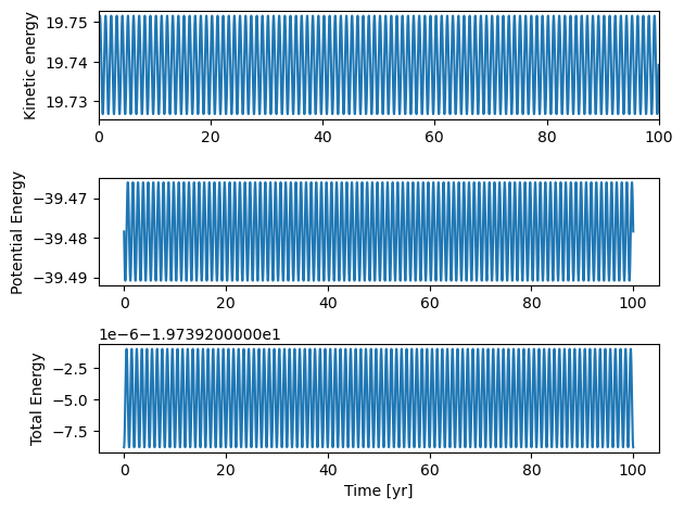
With the Euler-Cromer method, the only thing we need is to update the position at a time \(t+1\) with the update velocity from the same time. Thus, the change in the code is extremely simply, and energy is suddenly conserved. Note that the error runs like \(O(\Delta t)\) and this is why we see the larger oscillations. But within this oscillating energy envelope, we see that the energies swing between a max and a min value and never exceed these values.
# Common imports
import numpy as np
import pandas as pd
from math import *
import matplotlib.pyplot as plt
import os

# Where to save the figures and data files
PROJECT_ROOT_DIR = "Results"
FIGURE_ID = "Results/FigureFiles"
DATA_ID = "DataFiles/"

if not os.path.exists(PROJECT_ROOT_DIR):
    os.mkdir(PROJECT_ROOT_DIR)

if not os.path.exists(FIGURE_ID):
    os.makedirs(FIGURE_ID)

if not os.path.exists(DATA_ID):
    os.makedirs(DATA_ID)

def image_path(fig_id):
    return os.path.join(FIGURE_ID, fig_id)

def data_path(dat_id):
    return os.path.join(DATA_ID, dat_id)

def save_fig(fig_id):
    plt.savefig(image_path(fig_id) + ".png", format='png')

# Initial values, time step, positions and velocites

DeltaT = 0.0001
#set up arrays
tfinal = 100 # in years
n = ceil(tfinal/DeltaT)
# set up arrays for t, a, v, and x
t = np.zeros(n)
v = np.zeros((n,2))
r = np.zeros((n,2))

# setting up the kinetic, potential and total energy, note only functions of time
EKinetic = np.zeros(n)
EPotential = np.zeros(n)
ETotal = np.zeros(n)

# Initial conditions as compact 2-dimensional arrays


r0 = np.array([1.0,0.0])
v0 = np.array([0.0,2*pi])
r[0] = r0
v[0] = v0
Fourpi2 = 4*pi*pi
# Setting up variables for the calculation of energies
#  distance that defines rabs in potential energy
rabs0 = sqrt(sum(r[0]*r[0]))
#  Initial kinetic energy. Note that we skip the mass of the Earth here, that is MassEarth=1 in all codes
EKinetic[0] = 0.5*sum(v0*v0)
#  Initial potential energy
EPotential[0] = -4*pi*pi/rabs0
#  Initial total energy
ETotal[0] = EPotential[0]+EKinetic[0]
# Start integrating using Euler's method
for i in range(n-1):
    # Set up the acceleration
    # Here you could have defined your own function for this
    rabs = sqrt(sum(r[i]*r[i]))
    a =  -Fourpi2*r[i]/(rabs**3)
    # update velocity, time and position using Euler's forward method
    v[i+1] = v[i] + DeltaT*a
#   Only change when we add the Euler-Cromer method
    r[i+1] = r[i] + DeltaT*v[i+1]
    t[i+1] = t[i] + DeltaT
    EKinetic[i+1] = 0.5*sum(v[i+1]*v[i+1])
    EPotential[i+1] = -4*pi*pi/sqrt(sum(r[i+1]*r[i+1]))
    ETotal[i+1] = EPotential[i+1]+EKinetic[i+1]
# Plot energies as functions of time

fig, axs = plt.subplots(3, 1)
axs[0].plot(t, EKinetic)
axs[0].set_xlim(0, tfinal)
axs[0].set_ylabel('Kinetic energy')
axs[1].plot(t, EPotential)
axs[1].set_ylabel('Potential Energy')
axs[2].plot(t, ETotal)
axs[2].set_xlabel('Time [yr]')
axs[2].set_ylabel('Total Energy')
fig.tight_layout()
save_fig("EarthSunEulerCromer")
plt.show()
6.9.3. Adding the velocity Verlet method
Our final equations for the position and the velocity become then
and
Note well that the term \(a_{i+1}\) depends on the position at \(x_{i+1}\). This means that you need to calculate the position at the updated time \(t_{i+1}\) before the computing the next velocity. Note also that the derivative of the velocity at the time \(t_i\) used in the updating of the position can be reused in the calculation of the velocity update as well.
We can now easily add the Verlet method to our original code as
DeltaT = 0.001
#set up arrays
tfinal = 100
n = ceil(tfinal/DeltaT)
# set up arrays for t, a, v, and x
t = np.zeros(n)
v = np.zeros((n,2))
r = np.zeros((n,2))
# Initial conditions as compact 2-dimensional arrays
r0 = np.array([1.0,0.0])
v0 = np.array([0.0,2*pi])
r[0] = r0
v[0] = v0
Fourpi2 = 4*pi*pi

# setting up the kinetic, potential and total energy, note only functions of time
EKinetic = np.zeros(n)
EPotential = np.zeros(n)
ETotal = np.zeros(n)

# Setting up variables for the calculation of energies
#  distance that defines rabs in potential energy
rabs0 = sqrt(sum(r[0]*r[0]))
#  Initial kinetic energy. Note that we skip the mass of the Earth here, that is MassEarth=1 in all codes
EKinetic[0] = 0.5*sum(v0*v0)
#  Initial potential energy
EPotential[0] = -4*pi*pi/rabs0
#  Initial total energy
ETotal[0] = EPotential[0]+EKinetic[0]

# Start integrating using the Velocity-Verlet  method
for i in range(n-1):
    # Set up forces, air resistance FD, note now that we need the norm of the vecto
    # Here you could have defined your own function for this
    rabs = sqrt(sum(r[i]*r[i]))
    a =  -Fourpi2*r[i]/(rabs**3)
    # update velocity, time and position using the Velocity-Verlet method
    r[i+1] = r[i] + DeltaT*v[i]+0.5*(DeltaT**2)*a
    rabs = sqrt(sum(r[i+1]*r[i+1]))
    anew = -4*(pi**2)*r[i+1]/(rabs**3)
    v[i+1] = v[i] + 0.5*DeltaT*(a+anew)
    t[i+1] = t[i] + DeltaT
    EKinetic[i+1] = 0.5*sum(v[i+1]*v[i+1])
    EPotential[i+1] = -4*pi*pi/sqrt(sum(r[i+1]*r[i+1]))
    ETotal[i+1] = EPotential[i+1]+EKinetic[i+1]
# Plot energies as functions of time

fig, axs = plt.subplots(3, 1)
axs[0].plot(t, EKinetic)
axs[0].set_xlim(0, tfinal)
axs[0].set_ylabel('Kinetic energy')
axs[1].plot(t, EPotential)
axs[1].set_ylabel('Potential Energy')
axs[2].plot(t, ETotal)
axs[2].set_xlabel('Time [yr]')
axs[2].set_ylabel('Total Energy')
fig.tight_layout()
save_fig("EarthSunVelocityVerlet")
plt.show()
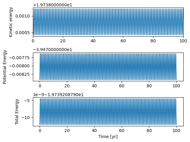
And we see that due to the smaller truncation error that energy conservation is improved as a function of time. Try out different time steps \(\Delta t\) and see if the results improve or worsen.
6.9.4. Exercise: Center-of-Mass and Relative Coordinates and Reference Frames
We define the two-body center-of-mass coordinate and relative coordinate by expressing the trajectories for \(\boldsymbol{r}_1\) and \(\boldsymbol{r}_2\) into the center-of-mass coordinate \(\boldsymbol{R}_{\rm cm}\)
and the relative coordinate
Here, we assume the two particles interact only with one another, so \(\boldsymbol{F}_{12}=-\boldsymbol{F}_{21}\) (where \(\boldsymbol{F}_{ij}\) is the force on \(i\) due to \(j\).
2a (5pt) Show that the equations of motion then become \(\ddot{\boldsymbol{R}}_{\rm cm}=0\) and \(\mu\ddot{\boldsymbol{r}}=\boldsymbol{F}_{12}\), with the reduced mass \(\mu=m_1m_2/(m_1+m_2)\).
The first expression simply states that the center of mass coordinate \(\boldsymbol{R}_{\rm cm}\) moves at a fixed velocity. The second expression can be rewritten in terms of the reduced mass \(\mu\).
Let us first start with some basic definitions. We have the center of mass coordinate \(\boldsymbol{R}\) defined as (for two particles)
where \(m_1\) and \(m_2\) are the masses of the two objects and \(\boldsymbol{r}_1\) and \(\boldsymbol{r}_2\) their respective positions defined according to a chosen origin. Here \(M=m_1+m_2\) is the total mass.
The relative position is defined as
and we then define \(\boldsymbol{r}_1\) and \(\boldsymbol{r}_2\) in terms of the relative and center of mass positions as
and
The total linear momentum is then defined as
where \(N=2\) in our case. With the above definition of the center of mass position, we see that we can rewrite the total linear momentum as (multiplying the center of mass position with \(M\))
This result is also an answer to a part of exercise 2b, see below.
The net force acting on the system is given by the time derivative of the linear momentum (assuming mass is time independent) and we have
The net force acting on the system is given by the sum of the forces acting on the two object, that is we have
In our case the forces are given by the internal forces only. The force acting on object \(1\) is thus \(\boldsymbol{F}_{12}\) and the one acting on object \(2\) is \(\boldsymbol{F}_{12}\). We have also defined that \(\boldsymbol{F}_{12}=-\boldsymbol{F}_{21}\). This means thar we have
which is what we wanted to show. The center of mass velocity is thus a constant of the motion. We could also define the so-called center of mass reference frame where we simply set \(\boldsymbol{R}=0\).
This has also another important consequence for our forces. If we assume that our force depends only on the positions, it means that the gradient of the potential with respect to the center of mass position is zero, that is
An alternative way is
The first expression simply states that the center of mass coordinate \(\boldsymbol{R}_{\rm cm}\) moves at a fixed velocity. The second expression can be rewritten in terms of the reduced mass \(\mu\).
Thus, one can treat the trajectory as a one-body problem where the reduced mass is \(\mu\), and a second trivial problem for the center of mass. The reduced mass is especially convenient when one is considering gravitational problems, as we have seen during the lectures of weeks 11-13.
2b (5pt) Show that the linear momenta for the center-of-mass \(\boldsymbol{P}\) motion and the relative motion \(\boldsymbol{q}\) are given by \(\boldsymbol{P}=M\dot{\boldsymbol{R}}_{\rm cm}\) with \(M=m_1+m_2\) and \(\boldsymbol{q}=\mu\dot{\boldsymbol{r}}\). The linear momentum of the relative motion is defined \(\boldsymbol{q} = (m_2\boldsymbol{p}_1-m_1\boldsymbol{p}_2)/(m_1+m_2)\).
In 2a we showed, as an intermediate step that the total linear momentum is given by
For the relative momentum \(\boldsymbol{q}\), we have that the time derivative of \(\boldsymbol{r}\) is
We now also that the momenta \(\boldsymbol{p}_1=m_1\dot{\boldsymbol{r}}_1\) and \(\boldsymbol{p}_2=m_2\dot{\boldsymbol{r}}_2\). Using these expressions we can rewrite
which we can rewrite as
and dividing both sides with \(M\) we have
Introducing the reduced mass \(\mu=m_1m_2/M\) we have finally
And \(\mu\dot{\boldsymbol{r}}\) defines the relative momentum \(\boldsymbol{q}=\mu\dot{\boldsymbol{r}}\).
When we introduce the Lagrangian formalism we will see that it is much easier to derive these equations.
2c (5pt) Show then that the kinetic energy for two objects can then be written as
Here we just need to use our definitions of kinetic energy in terms of the coordinates \(\boldsymbol{r}_1\) and \(\boldsymbol{r}_2\).
We have that
and with \(\boldsymbol{p}_1=m_1\dot{\boldsymbol{r}}_1\) and \(\boldsymbol{p}_2=m_2\dot{\boldsymbol{r}}_2\) and using
and
we obtain (after squaring the expressions for \(\dot{\boldsymbol{r}}_1\) and \(\dot{\boldsymbol{r}}_2\)) we have
which we simplify to
which is what we wanted to show.
2d (5pt) Show that the total angular momentum for two-particles in the center-of-mass frame \(\boldsymbol{R}=0\), is given by
Here we need again that
and we then define \(\boldsymbol{r}_1\) and \(\boldsymbol{r}_2\) in terms of the relative and center of mass positions with \(\boldsymbol{R}=0\)
and
The angular momentum (the total one) is the sum of the individual angular momenta (see homework 4) and we have
and using that \(m_1\dot{\boldsymbol{r}}_1=\boldsymbol{p}_1\) and \(m_2\dot{\boldsymbol{r}}_2=\boldsymbol{p}_2\) we have
Inserting the equations for \(\boldsymbol{r}_1\) and \(\boldsymbol{r}_2\) in terms of the relative motion, we have
We see that can rewrite this equation as
which is what we wanted to derive.
6.9.5. Exercise: Conservation of Energy
The equations of motion in the center-of-mass frame in two dimensions with \(x=r\cos{(\phi)}\) and \(y=r\sin{(\phi)}\) and \(r\in [0,\infty)\), \(\phi\in [0,2\pi]\) and \(r=\sqrt{x^2+y^2}\) are given by
and
Here \(V(r)\) is any central force which depends only on the relative coordinate.
1a (5pt) Show that you can rewrite the radial equation in terms of an effective potential \(V_{\mathrm{eff}}(r)=V(r)+L^2/(2\mu r^2)\).
Here we use that
and rewrite the above equation of motion as
If we now define an effective potential
we can rewrite our equation of motion in terms of
The addition due to the angular momentum comes from the kinetic energy when we rewrote it in terms of polar coordinates. It introduces a so-called centrifugal barrier due to the angular momentum. This centrifugal barrier pushes the object farther away from the origin.
Alternatively,
Integrating we obtain
Imposing the extra condition that \(V_{\text{eff}}(r\rightarrow \infty) = V(r\rightarrow \infty)\),
Write out the final differential equation for the radial degrees of freedom when we specify that \(V(r)=-\alpha/r\). Plot the effective potential. You can choose values for \(\alpha\) and \(L\) and discuss (see Taylor section 8.4 and example 8.2) the physics of the system for two energies, one larger than zero and one smaller than zero. This is similar to what you did in the first midterm, except that the potential is different.
We insert now the explicit potential form \(V(r)=-\alpha/r\). This gives us the following equation of motion
The following code plots this effective potential for a simple choice of parameters, with a standard gravitational potential \(-\alpha/r\). Here we have chosen \(L=m=\alpha=1\).
# Common imports
import numpy as np
from math import *
import matplotlib.pyplot as plt

Deltax = 0.01
#set up arrays
xinitial = 0.3
xfinal = 5.0
alpha = 1.0   # spring constant
m = 1.0   # mass, you can change these
AngMom = 1.0  #  The angular momentum
n = ceil((xfinal-xinitial)/Deltax)
x = np.zeros(n)
for i in range(n):
    x[i] = xinitial+i*Deltax
V = np.zeros(n)
V = -alpha/x+0.5*AngMom*AngMom/(m*x*x)
# Plot potential
fig, ax = plt.subplots()
ax.set_xlabel('r[m]')
ax.set_ylabel('V[J]')
ax.plot(x, V)
fig.tight_layout()
plt.show()
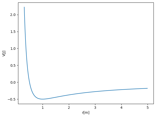
If we select a potential energy below zero (and not necessarily one which corresponds to the minimum point), the object will oscillate between two values of \(r\), a value \(r_{\mathrm{min}}\) and a value \(r_{\mathrm{max}}\). We can assume that for example the kinetic energy is zero at these two points. The object will thus oscillate back and forth between these two points. As we will see in connection with the solution of the equations of motion, this case corresponds to elliptical orbits. If we select \(r\) equal to the minimum of the potential and use initial conditions for the velocity that correspond to circular motion, the object will have a constant value of \(r\) given by the value at the minimum and the orbit is a circle.
If we select a potential energy larger than zero, then, since the kinetic energy is always larger or equal to zero, the object will move away from the origin. See also the discussion in Taylor, sections 8.4-8.6.
6.9.6. Exercise: Harmonic oscillator again
Consider a particle of mass \(m\) in a \(2\)-dimensional harmonic oscillator with potential
We assume the orbit has a final non-zero angular momentum \(L\). The effective potential looks like that of a harmonic oscillator for large \(r\), but for small \(r\), the centrifugal potential repels the particle from the origin. The combination of the two potentials has a minimum for at some radius \(r_{\rm min}\).
Set up the effective potential and plot it. Find \(r_{\rm min}\) and \(\dot{\phi}\). Show that the latter is given by \(\dot{\phi}=\sqrt{k/m}\). At \(r_{\rm min}\) the particle does not accelerate and \(r\) stays constant and the motion is circular. With fixed \(k\) and \(m\), which parameter can we adjust to change the value of \(r\) at \(r_{\rm min}\)?
We consider the effective potential. The radius of a circular orbit is at the minimum of the potential (where the effective force is zero). The potential is plotted here with the parameters \(k=m=1.0\) and \(L=1.0\).
# Common imports
import numpy as np
from math import *
import matplotlib.pyplot as plt

Deltax = 0.01
#set up arrays
xinitial = 0.5
xfinal = 3.0
k = 1.0   # spring constant
m = 1.0   # mass, you can change these
AngMom = 1.0  #  The angular momentum
n = ceil((xfinal-xinitial)/Deltax)
x = np.zeros(n)
for i in range(n):
    x[i] = xinitial+i*Deltax
V = np.zeros(n)
V = 0.5*k*x*x+0.5*AngMom*AngMom/(m*x*x)
# Plot potential
fig, ax = plt.subplots()
ax.set_xlabel('r[m]')
ax.set_ylabel('V[J]')
ax.plot(x, V)
fig.tight_layout()
plt.show()
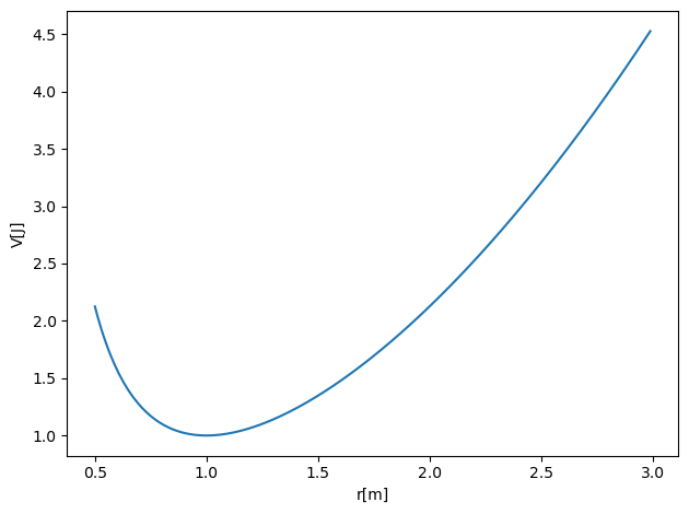
We have an effective potential
The effective potential looks like that of a harmonic oscillator for large \(r\), but for small \(r\), the centrifugal potential repels the particle from the origin. The combination of the two potentials has a minimum for at some radius \(r_{\rm min}\).
For particles at \(r_{\rm min}\) with \(\dot{r}=0\), the particle does not accelerate and \(r\) stays constant, i.e. a circular orbit. The radius of the circular orbit can be adjusted by changing the angular momentum \(L\).
For the above parameters this minimum is at \(r_{\rm min}=1\).
Now consider small vibrations about \(r_{\rm min}\). The effective spring constant is the curvature of the effective potential. Use the curvature at \(r_{\rm min}\) to find the effective spring constant (hint, look at exercise 4 in homework 6) \(k_{\mathrm{eff}}\). Show also that \(\omega=\sqrt{k_{\mathrm{eff}}/m}=2\dot{\phi}\)
Because the radius oscillates with twice the angular frequency, the orbit has two places where \(r\) reaches a minimum in one cycle. This differs from the inverse-square force where there is one minimum in an orbit. One can show that the orbit for the harmonic oscillator is also elliptical, but in this case the center of the potential is at the center of the ellipse, not at one of the foci.
The solution to the equations of motion in Cartesian coordinates is simple. The \(x\) and \(y\) equations of motion separate, and we have \(\ddot{x}=-kx/m\) and \(\ddot{y}=-ky/m\). The harmonic oscillator is indeed a system where the degrees of freedom separate and we can find analytical solutions. Define a natural frequency \(\omega_0=\sqrt{k/m}\) and show that (where \(A\), \(B\), \(C\) and \(D\) are arbitrary constants defined by the initial conditions)
The solution is also simple to write down exactly in Cartesian coordinates. The \(x\) and \(y\) equations of motion separate,
We know from our studies of the harmonic oscillator that the general solution can be expressed as
With the solutions for \(x\) and \(y\), and \(r^2=x^2+y^2\) and the definitions \(\alpha=\frac{A^2+B^2+C^2+D^2}{2}\), \(\beta=\frac{A^2-B^2+C^2-D^2}{2}\) and \(\gamma=AB+CD\), show that
with
We start with \(r^2 & = x^2+y^2\) and square the above analytical solutions and after some exciting algebraic manipulations we arrive at
which is what we wanted to show.
6.9.7. Exercise: Numerical Solution of the Harmonic Oscillator
Using the code we developed in homeworks 5 and/or 6 for the Earth-Sun system, we can solve the above harmonic oscillator problem in two dimensions using our code from this homework. We need however to change the acceleration from the gravitational force to the one given by the harmonic oscillator potential.
3a (20pt) Use for example the code in the exercise set to set up the acceleration and use the initial conditions fixed by for example \(r_{\rm min}\) from exercise 2. Which value should the initial velocity take if you place yourself at \(r_{\rm min}\) and you require a circular motion? Hint: see the first midterm, part 2. There you used the centripetal acceleration.
Instead of solving the equations in the cartesian frame we will now rewrite the above code in terms of the radial degrees of freedom only. Our differential equation is now
and
3b (20pt) We will use \(r_{\rm min}\) to fix a value of \(L\), as seen in exercise 2. This fixes also \(\dot{\phi}\). Write a code which now implements the radial equation for \(r\) using the same \(r_{\rm min}\) as you did in 3a. Compare the results with those from 3a with the same initial conditions. Do they agree? Use only one set of initial conditions.
The code here finds the solution for \(x\) and \(y\) using the code we developed in homework 5 and 6 and the midterm. Note that this code is tailored to run in Cartesian coordinates. There is thus no angular momentum dependent term.
Here we have chosen initial conditions that correspond to the minimum of the effective potential \(r_{\mathrm{min}}\). We have chosen \(x_0=r_{\mathrm{min}}\) and \(y_0=0\). Similarly, we use the centripetal acceleration to determine the initial velocity so that we have a circular motion (see back to the last question of the midterm). This means that we set the centripetal acceleration \(v^2/r\) equal to the force from the harmonic oscillator \(-k\boldsymbol{r}\). Taking the magnitude of \(\boldsymbol{r}\) we have then \(v^2/r=k/mr\), which gives \(v=\pm\omega_0r\).
Since the code here solves the equations of motion in cartesian coordinates and the harmonic oscillator potential leads to forces in the \(x\)- and \(y\)-directions that are decoupled, we have to select the initial velocities and positions so that we don’t get that for example \(y(t)=0\).
We set \(x_0\) to be different from zero and \(v_{y0}\) to be different from zero.
# Common imports
import numpy as np
import pandas as pd
from math import *
import matplotlib.pyplot as plt
import os

# Where to save the figures and data files
PROJECT_ROOT_DIR = "Results"
FIGURE_ID = "Results/FigureFiles"
DATA_ID = "DataFiles/"

if not os.path.exists(PROJECT_ROOT_DIR):
    os.mkdir(PROJECT_ROOT_DIR)

if not os.path.exists(FIGURE_ID):
    os.makedirs(FIGURE_ID)

if not os.path.exists(DATA_ID):
    os.makedirs(DATA_ID)

def image_path(fig_id):
    return os.path.join(FIGURE_ID, fig_id)

def data_path(dat_id):
    return os.path.join(DATA_ID, dat_id)

def save_fig(fig_id):
    plt.savefig(image_path(fig_id) + ".png", format='png')

DeltaT = 0.001
#set up arrays
tfinal = 10.0
n = ceil(tfinal/DeltaT)
# set up arrays
t = np.zeros(n)
v = np.zeros((n,2))
r = np.zeros((n,2))
radius = np.zeros(n)
# Constants of the model
k = 1.0   # spring constant
m = 1.0   # mass, you can change these
omega02 = k/m  # Frequency
AngMom = 1.0  #  The angular momentum
# Potential minimum
rmin = (AngMom*AngMom/k/m)**0.25
# Initial conditions as compact 2-dimensional arrays, x0=rmin and y0 = 0
x0 = rmin; y0= 0.0
r0 = np.array([x0,y0])
vy0 = sqrt(omega02)*rmin; vx0 = 0.0
v0 = np.array([vx0,vy0])
r[0] = r0
v[0] = v0
# Start integrating using the Velocity-Verlet  method
for i in range(n-1):
    # Set up the acceleration
    a =  -r[i]*omega02
    # update velocity, time and position using the Velocity-Verlet method
    r[i+1] = r[i] + DeltaT*v[i]+0.5*(DeltaT**2)*a
    anew = -r[i+1]*omega02
    v[i+1] = v[i] + 0.5*DeltaT*(a+anew)
    t[i+1] = t[i] + DeltaT
# Plot position as function of time
radius = np.sqrt(r[:,0]**2+r[:,1]**2)
fig, ax = plt.subplots(3,1)
ax[0].set_xlabel('time')
ax[0].set_ylabel('radius squared')
ax[0].plot(t,r[:,0]**2+r[:,1]**2)
ax[1].set_xlabel('time')
ax[1].set_ylabel('x position')
ax[1].plot(t,r[:,0])
ax[2].set_xlabel('time')
ax[2].set_ylabel('y position')
ax[2].plot(t,r[:,1])

fig.tight_layout()
save_fig("2DimHOVV")
plt.show()
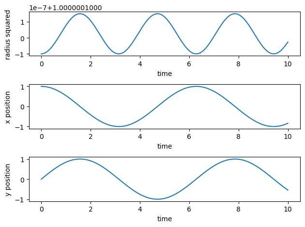
We see that the radius (to within a given error), we obtain a constant radius.
The following code shows first how we can solve this problem using the radial degrees of freedom only. Here we need to add the explicit centrifugal barrier. Note that the variable \(r\) depends only on time. There is no \(x\) and \(y\) directions since we have transformed the equations to polar coordinates.
DeltaT = 0.01
#set up arrays
tfinal = 10.0
n = ceil(tfinal/DeltaT)
# set up arrays for t, v and r
t = np.zeros(n)
v = np.zeros(n)
r = np.zeros(n)
E = np.zeros(n)
# Constants of the model
AngMom = 1.0  #  The angular momentum
m = 1.0
k = 1.0
omega02 = k/m
c1 = AngMom*AngMom/(m*m)
c2 = AngMom*AngMom/m
rmin = (AngMom*AngMom/k/m)**0.25
# Initial conditions
r0 = rmin
v0 = 0.0
r[0] = r0
v[0] = v0
E[0] = 0.5*m*v0*v0+0.5*k*r0*r0+0.5*c2/(r0*r0)
# Start integrating using the Velocity-Verlet  method
for i in range(n-1):
    # Set up acceleration
    a = -r[i]*omega02+c1/(r[i]**3)
    # update velocity, time and position using the Velocity-Verlet method
    r[i+1] = r[i] + DeltaT*v[i]+0.5*(DeltaT**2)*a
    anew = -r[i+1]*omega02+c1/(r[i+1]**3)
    v[i+1] = v[i] + 0.5*DeltaT*(a+anew)
    t[i+1] = t[i] + DeltaT
    E[i+1] = 0.5*m*v[i+1]*v[i+1]+0.5*k*r[i+1]*r[i+1]+0.5*c2/(r[i+1]*r[i+1])
    # Plot position as function of time
fig, ax = plt.subplots(2,1)
ax[0].set_xlabel('time')
ax[0].set_ylabel('radius')
ax[0].plot(t,r)
ax[1].set_xlabel('time')
ax[1].set_ylabel('Energy')
ax[1].plot(t,E)
save_fig("RadialHOVV")
plt.show()
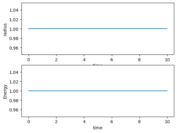
6.9.8. Exercise: Equations for an ellipse
Consider an ellipse defined by the sum of the distances from the two foci being \(2D\), which expressed in a Cartesian coordinates with the middle of the ellipse being at the origin becomes
Here the two foci are at \((a,0)\) and \((-a,0)\). Show that this form is can be written as
We start by squaring the two sides and, again, after some exciting algebraic manipulations we arrive at
where the last line is indeed the equation for an ellipse.
6.9.9. Exercise: Attractive Potential
Consider a particle in an attractive potential
The quantity \(r\) is the absolute value of the relative position. We will use the reduced mass \(\mu\) and the angular momentum \(L\), as discussed during the lectures. With the transformation of a two-body problem to the center-of-mass frame, the actual equations look like an effective one-body problem. The energy of the system is \(E\) and the minimum of the effective potential is \(r_{\rm min}\).
The analytical solution to the radial equation of motion is
Find the value of \(A\). Hint: Use the fact that at \(r_{\rm min}\) there is no radial kinetic energy and \(E=-\alpha/r_{\rm min}+L^2/2mr_{\rm min}^2\).
At \(r_{\mathrm{min}}\) and \(r_{\mathrm{max}}\) , all the kinetic energy is stored in the velocity in the direction perpendicular to \(r\) since the radial velocity is set to zero . We can calculate using angular momentum and from there, find 𝐴 in terms of the energy \(E\) which is constant. But first, we need to find \(r_{\mathrm{min}}\) from the conservation of energy (noting that the radial velocity \(\ddot{r}\) at the mininum is zero):
Since we’re looking for the minimum, the ± sign must be negative (then 𝑟min will not be negative since 𝐸<0 ). Therefore, we have
6.9.10. Exercise: Inverse-square force
Consider again the same effective potential as in the previous exercise. This leads to an attractive inverse-square-law force, \(F=-\alpha/r^2\). Consider a particle of mass \(m\) with angular momentum \(L\). Taylor sections 8.4-8.7 are relevant background material. See also the harmonic oscillator potential from hw8. The equation of motion for the radial degrees of freedom is (see also hw8) in the center-of-mass frame in two dimensions with \(x=r\cos{(\phi)}\) and \(y=r\sin{(\phi)}\) and \(r\in [0,\infty)\), \(\phi\in [0,2\pi]\) and \(r=\sqrt{x^2+y^2}\) are given by
and
Here \(V(r)\) is any central force which depends only on the relative coordinate.
Find the radius of a circular orbit by solving for the position of the minimum of the effective potential.
At the minimum, the radial velocity is zero and it is only the centripetal velocity which is nonzero. This implies that \(\ddot{r}=0\). What is the angular frequency, \(\dot{\theta}\), of the orbit? Solve this by setting \(\ddot{r}=0=F/m+\dot{\theta}^2r\).
Find the effective spring constant for the particle at the minimum.
We have shown in class that from the taylor expansion, we have
Therefore, all we have to do is find the second derivative of \(V_{\text{eff}}\) around the minimum point of \(V_{\text{eff}}\) where \(\dot{r} = \ddot{r} = 0\).
What is the angular frequency for small vibrations about the minimum? How does this compare with the answer to (3b)?
For small deviations \(\delta r\) of \(r\),
The solution of this differential equation is of the form
where
This is in fact equal to the expression for \(\dot{\theta}\). This means that small perturbations oscillate in sync with the orbit and this traces out an ellipse with a very small eccentricity, a very nice physical result.
6.9.11. Exercise: Inverse-square force again
Consider again a particle of mass \(m\) in the same attractive potential, \(U(r)=-\alpha/r\), with angular momentum \(L\) with just the right energy so that
where \(A\) comes from the expression
The trajectory can then be rewritten as
Show that for this case the total energy \(E\) approaches zero.
With zero energy \(E=0\), write this trajectory in a more recognizable parabolic form, that is express \(x_0\) and \(R\) in terms of \(r_0\) using
We have that
Using the general solution with eccintricity \(\epsilon=1\), we have
and multiplying both sides with \(1+\cos\theta\) and using that \(x=r\cos\theta\),
and using that \(r^2=x^2+y^2\), we square both sides
leading to
and using that we defined
we divide by \(2c\) and we get the final answer
6.9.12. Exercise: Parabolic and hyperbolic orbits
The solution to the radial function for an inverse-square-law force, see for example Taylor equation (8.59) or the equation above, is
For \(\epsilon=1\) (or the energy \(E=0\)) the orbit reduces to a parabola as we saw in the previous exercise, while for \(\epsilon > 1\) (or energy positive) the orbit becomes a hyperbola. The equation for a hyperbola in Cartesian coordinates is
For a hyperbola, identify the constants \(\alpha\), \(\beta\) and \(\delta\) in terms of the constants \(c\) and \(\epsilon\) for \(r(\phi)\).
Here \(\epsilon>1\). We use our equation for \(r\), multiply with the denominator \(1+\epsilon\cos\phi\) on both sides and have
use \(x=r\cos\phi\) and square and use that \(r^2=x^2+y^2\) and we have
and reorder
We complete the square in \(x\) by adding and subtracting on both sides \(\epsilon^2c^2/(\epsilon^2-1)\) and we obtain
Here we have defined
and introducing the constants
and
we can rewrite the above equation as
which is nothing but the equation for a hyperbola.
6.9.13. Exercise: Testing orbit types
In this exercise we can use the program for \(r(\phi)\) we developed in hw8. We will use an inverse-square-law force as in the previous four exercises. The aim is to see that the orbits we get for \(E<0\) become ellipses (or circles), parabola for \(E=0\) and hyperbola for \(E>0\). An example code is shown here.
Here we have defined the constants \(L=m=\alpha=1\). Feel free to set new values. You need also to set the initial conditions in order to study the different types of orbits. It may be useful to plot the potential here and find the values for the initial conditions that fit \(E<0\), \(E=0\) and \(E>0\).
# Common imports
import numpy as np
import pandas as pd
from math import *
import matplotlib.pyplot as plt
# Simple Gravitational Force   -alpha/r

DeltaT = 0.01
#set up arrays
tfinal = 100.0
n = ceil(tfinal/DeltaT)
# set up arrays for t, v and r
t = np.zeros(n)
v = np.zeros(n)
r = np.zeros(n)
# Constants of the model, setting all variables to one for simplicity
alpha = 1.0
AngMom = 1.0  #  The angular momentum
m = 1.0  # scale mass to one
c1 = AngMom*AngMom/(m*m)
c2 = AngMom*AngMom/m
# You need to specify the initial conditions
# Here we have chosen the conditions which lead to circular orbit and thereby a constant r
r0 = (AngMom*AngMom/m/alpha)
v0 = 0.0
r[0] = r0
v[0] = v0
# Start integrating using the Velocity-Verlet  method
for i in range(n-1):
    # Set up acceleration
    a = -alpha/(r[i]**2)+c1/(r[i]**3)
    # update velocity, time and position using the Velocity-Verlet method
    r[i+1] = r[i] + DeltaT*v[i]+0.5*(DeltaT**2)*a
    anew = -alpha/(r[i+1]**2)+c1/(r[i+1]**3)
    v[i+1] = v[i] + 0.5*DeltaT*(a+anew)
    t[i+1] = t[i] + DeltaT
    # Plot position as function of time
fig, ax = plt.subplots(2,1)
ax[0].set_xlabel('time')
ax[0].set_ylabel('radius')
ax[0].plot(t,r)
ax[1].set_xlabel('time')
ax[1].set_ylabel('Velocity')
ax[1].plot(t,v)

plt.show()

Run your code and study and discuss the situations where you have elliptical, parabolic and hyperbolic orbits. Discuss the physics of these cases. The results from the four previous exercises 4 may be useful here. In the code here we have chosen initial conditions which correspond to circular motion. This corresponds to
Note well that the velocity is now the radial velocity. If we want to study the angular velocity we would need to add the equations for this quantity. The solution to exercises 1-4 give you the minimum \(r\) values needed to find the elliptical, parabolic and hyperbolic orbits. For elliptical orbits you should have \(\frac{L^2}{2m\alpha} < r_{\mathrm{min}} <\frac{L^2}{m\alpha}\). For parabolic orbits \(r_{\mathrm{min}} =\frac{L^2}{m\alpha}\) and for hyperbolic orbits we have \(0<r_{\mathrm{min}} <\frac{L^2}{m\alpha}\). Try out these different initial conditions in order to test these different types of motion.
6.9.14. Exercise: New reference frame
Show that if one transforms to a reference frame where the total momentum is zero, \(\boldsymbol{p}_1=-\boldsymbol{p}_2\), that the relative momentum \(\boldsymbol{q}\) corresponds to either \(\boldsymbol{p}_1\) or \(-\boldsymbol{p}_2\). This means that in this frame the magnitude of \(\boldsymbol{q}\) is one half the magnitude of \(\boldsymbol{p}_1-\boldsymbol{p}_2\).
6.9.15. Exercise: Center of mass and relative coordinates
Given the center of mass and relative coordinates \(\boldsymbol{R}\) and \(\boldsymbol{r}\), respectively, for particles of mass \(m_1\) and \(m_2\), find the coordinates \(\boldsymbol{r}_1\) and \(\boldsymbol{r}_2\) in terms of the masses, \(\boldsymbol{R}\) and \(\boldsymbol{r}\).
6.9.16. Exercise: Two-body problems
Consider a particle of mass \(m\) moving in a potential
where \(\alpha\) is a constant.
(a) If the particle is moving in a circular orbit of radius \(R\), find the angular frequency \(\dot{\theta}\). Solve this by setting \(F=-m\dot{\theta}^2r\) (force and acceleration point inward).
(b) Express the angular momentum \(L\) in terms of the constant \(\alpha\), the mass \(m\) and the radius \(R\). Also express \(R\) in terms of \(L\), \(\alpha\) and \(m\).
(c) Sketch the effective radial potential, \(V_{\rm eff}(r)\), for a particle with angular momentum \(L\). (No longer necessarily moving in a circular orbit.)
(d) Find the position of the minimum of \(V_{\rm eff}\) in terms of \(L\), \(\alpha\) and \(m\), then compare to the result of (b).
(e) What is the effective spring constant for a particle at the minimum of \(V_{\rm eff}\)? Express your answer in terms of \(L\), \(m\) and \(\alpha\).
(f) What is the angular frequency, \(\omega\), for small oscillations of \(r\) about the \(R_{\rm min}\)? Express your answer in terms of \(\dot{\theta}\) from part (3a).