Work, Energy, Momentum and Conservation laws
Contents
4. Work, Energy, Momentum and Conservation laws
In the previous three chapters we have shown how to use Newton’s laws of motion to determine the motion of an object based on the forces acting on it. For two of the cases there is an underlying assumption that we can find an analytical solution to a continuous problem. With a continuous problem we mean a problem where the various variables can take any value within a finite or infinite interval.
Unfortunately, in many cases we cannot find an exact solution to the equations of motion we get from Newton’s second law. The numerical approach, where we discretize the continuous problem, allows us however to study a much richer set of problems. For problems involving Newton’s laws and the various equations of motion we encounter, solving the equations numerically, is the standard approach.
It allows us to focus on the underlying forces. Often we end up using the same numerical algorithm for different problems.
Here we introduce a commonly used technique that allows us to find the velocity as a function of position without finding the position as a function of time—an alternate form of Newton’s second law. The method is based on a simple principle: Instead of solving the equations of motion directly, we integrate the equations of motion. Such a method is called an integration method.
This allows us also to introduce the work-energy theorem. This theorem allows us to find the velocity as a function of position for an object even in cases when we cannot solve the equations of motion. This introduces us to the concept of work and kinetic energy, an energy related to the motion of an object.
And finally, we will link the work-energy theorem with the principle of conservation of energy.
4.1. The Work-Energy Theorem
Let us define the kinetic energy \(K\) with a given velocity \(\boldsymbol{v}\)
where \(m\) is the mass of the object we are considering. We assume also that there is a force \(\boldsymbol{F}\) acting on the given object
with \(\boldsymbol{r}\) the position and \(t\) the time. In general we assume the force is a function of all these variables. Many of the more central forces in Nature however, depende only on the position. Examples are the gravitational force and the force derived from the Coulomb potential in electromagnetism.
Let us study the derivative of the kinetic energy with respect to time \(t\). Its continuous form is
Using our results from exercise 3 of homework 1, we can write the derivative of a vector dot product as
We know also that the acceleration is defined as
We can then rewrite the equation for the derivative of the kinetic energy as
where we defined the velocity as the derivative of the position with respect to time.
Let us now discretize the above equation by letting the instantaneous terms be replaced by a discrete quantity, that is we let \(dK\rightarrow \Delta K\), \(dt\rightarrow \Delta t\), \(d\boldsymbol{r}\rightarrow \Delta \boldsymbol{r}\) and \(d\boldsymbol{v}\rightarrow \Delta \boldsymbol{v}\).
We have then
or by multiplying out \(\Delta t\) we have
We define this quantity as the work done by the force \(\boldsymbol{F}\) during the displacement \(\Delta \boldsymbol{r}\). If we study the dimensionality of this problem we have mass times length squared divided by time squared, or just dimension energy.
If we now define a series of such displacements \(\Delta\boldsymbol{r}\) we have a difference in kinetic energy at a final position \(\boldsymbol{r}_n\) and an initial position \(\boldsymbol{r}_0\) given by
where \(\boldsymbol{F}_i\) are the forces acting at every position \(\boldsymbol{r}_i\).
The work done by acting with a force on a set of displacements can then be as expressed as the difference between the initial and final kinetic energies.
This defines the work-energy theorem.
If we take the limit \(\Delta \boldsymbol{r}\rightarrow 0\), we can rewrite the sum over the various displacements in terms of an integral, that is
This integral defines a path integral since it will depend on the given path we take between the two end points. We will replace the limits with the symbol \(c\) in order to indicate that we take a specific countour in space when the force acts on the system. That is the work \(W_{n0}\) between two points \(\boldsymbol{r}_n\) and \(\boldsymbol{r}_0\) is labeled as
Note that if the force is perpendicular to the displacement, then the force does not affect the kinetic energy.
Let us now study some examples of forces and how to find the velocity from the integration over a given path.
Thereafter we study how to evaluate an integral numerically.
In order to study the work- energy, we will normally need to perform a numerical integration, unless we can integrate analytically. Here we present some of the simpler methods such as the rectangle rule, the trapezoidal rule and higher-order methods like the Simpson family of methods.
4.1.1. Example of an Electron moving along a Surface
As an example, let us consider the following case. We have classical electron which moves in the \(x\)-direction along a surface. The force from the surface is
The constant \(b\) represents the distance between atoms at the surface of the material, \(F_0\) is a constant and \(x\) is the position of the electron.
Using the work-energy theorem we can find the work \(W\) done when moving an electron from a position \(x_0\) to a final position \(x\) through the integral
which results in
If we now use the work-energy theorem we can find the the velocity at a final position \(x\) by setting up the differences in kinetic energies between the final position and the initial position \(x_0\).
We have that the work done by the force is given by the difference in kinetic energies as
and labeling \(v(x_0)=v_0\) (and assuming we know the initial velocity) we have
Choosing \(x_0=0\)m and \(v_0=0\)m/s we can simplify the above equation to
4.1.2. Harmonic Oscillations
Another well-known force (and we will derive when we come to Harmonic Oscillations) is the case of a sliding block attached to a wall through a spring. The block is attached to a spring with spring constant \(k\). The other end of the spring is attached to the wall at the origin \(x=0\). We assume the spring has an equilibrium length \(L_0\).
The force \(F_x\) from the spring on the block is then
The position \(x\) where the spring force is zero is called the equilibrium position. In our case this is \(x=L_0\).
We can now compute the work done by this force when we move our block from an initial position \(x_0\) to a final position \(x\)
If we now bring back the definition of the work-energy theorem in terms of the kinetic energy we have
which we rewrite as
What does this mean? The total energy, which is the sum of potential and kinetic energy, is conserved. Wow, this sounds interesting. We will analyze this next week in more detail when we study energy, momentum and angular momentum conservation.
4.2. Numerical Integration
Let us now see how we could have solved the above integral numerically.
There are several numerical algorithms for finding an integral numerically. The more familiar ones like the rectangular rule or the trapezoidal rule have simple geometric interpretations.
Let us look at the mathematical details of what are called equal-step methods, also known as Newton-Cotes quadrature.
4.3. Newton-Cotes Quadrature or equal-step methods
The integral
has a very simple meaning. The integral is the area enscribed by the function \(f(x)\) starting from \(x=a\) to \(x=b\). It is subdivided in several smaller areas whose evaluation is to be approximated by different techniques. The areas under the curve can for example be approximated by rectangular boxes or trapezoids.
In considering equal step methods, our basic approach is that of approximating a function \(f(x)\) with a polynomial of at most degree \(N-1\), given \(N\) integration points. If our polynomial is of degree \(1\), the function will be approximated with \(f(x)\approx a_0+a_1x\).
The algorithm for these integration methods is rather simple, and the number of approximations perhaps unlimited!
Choose a step size \(h=(b-a)/N\) where \(N\) is the number of steps and \(a\) and \(b\) the lower and upper limits of integration.
With a given step length we rewrite the integral as
The strategy then is to find a reliable polynomial approximation for \(f(x)\) in the various intervals. Choosing a given approximation for \(f(x)\), we obtain a specific approximation to the integral.
With this approximation to \(f(x)\) we perform the integration by computing the integrals over all subintervals.
One possible strategy then is to find a reliable polynomial expansion for \(f(x)\) in the smaller subintervals. Consider for example evaluating
which we rewrite as
We have chosen a midpoint \(x_0\) and have defined \(x_0=a+h\).
4.3.1. The rectangle method
A very simple approach is the so-called midpoint or rectangle method. In this case the integration area is split in a given number of rectangles with length \(h\) and height given by the mid-point value of the function. This gives the following simple rule for approximating an integral
where \(f(x_{i-1/2})\) is the midpoint value of \(f\) for a given rectangle. We will discuss its truncation error below. It is easy to implement this algorithm, as shown below
The correct mathematical expression for the local error for the rectangular rule \(R_i(h)\) for element \(i\) is
and the global error reads
where \(R_h\) is the result obtained with rectangular rule and \(\xi \in [a,b]\).
We go back to our simple example above and set \(F_0=b=1\) and choose \(x_0=0\) and \(x=1/2\), and have
The code here computes the integral using the rectangle rule and \(n=100\) integration points we have a relative error of \(10^{-5}\).
from math import sin, pi
import numpy as np
from sympy import Symbol, integrate
# function for the Rectangular rule
def Rectangular(a,b,f,n):
   h = (b-a)/float(n)
   s = 0
   for i in range(0,n,1):
       x = (i+0.5)*h
       s = s+ f(x)
   return h*s
# function to integrate
def function(x):
    return sin(2*pi*x)
# define integration limits and integration points
a = 0.0; b = 0.5;
n = 100
Exact = 1./pi
print("Relative error= ", abs( (Rectangular(a,b,function,n)-Exact)/Exact))
Relative error= 4.112453549290521e-05
4.3.2. The trapezoidal rule
The other integral gives
and adding up we obtain
which is the well-known trapezoidal rule. Concerning the error in the approximation made, \(O(h^3)=O((b-a)^3/N^3)\), you should note that this is the local error. Since we are splitting the integral from \(a\) to \(b\) in \(N\) pieces, we will have to perform approximately \(N\) such operations.
This means that the global error goes like \(\approx O(h^2)\). The trapezoidal reads then
with a global error which goes like \(O(h^2)\).
Hereafter we use the shorthand notations \(f_{-h}=f(x_0-h)\), \(f_{0}=f(x_0)\) and \(f_{h}=f(x_0+h)\).
The correct mathematical expression for the local error for the trapezoidal rule is
and the global error reads
where \(T_h\) is the trapezoidal result and \(\xi \in [a,b]\).
The trapezoidal rule is easy to implement numerically through the following simple algorithm
Choose the number of mesh points and fix the step length.
calculate \(f(a)\) and \(f(b)\) and multiply with \(h/2\).
Perform a loop over \(n=1\) to \(n-1\) (\(f(a)\) and \(f(b)\) are known) and sum up the terms \(f(a+h) +f(a+2h)+f(a+3h)+\dots +f(b-h)\). Each step in the loop corresponds to a given value \(a+nh\).
Multiply the final result by \(h\) and add \(hf(a)/2\) and \(hf(b)/2\).
We use the same function and integrate now using the trapoezoidal rule.
import numpy as np
from sympy import Symbol, integrate
# function for the trapezoidal rule
def Trapez(a,b,f,n):
   h = (b-a)/float(n)
   s = 0
   x = a
   for i in range(1,n,1):
       x = x+h
       s = s+ f(x)
   s = 0.5*(f(a)+f(b)) +s
   return h*s
# function to integrate
def function(x):
    return sin(2*pi*x)
# define integration limits and integration points
a = 0.0; b = 0.5;
n = 100
Exact = 1./pi
print("Relative error= ", abs( (Trapez(a,b,function,n)-Exact)/Exact))
Relative error= 8.224805627923717e-05
4.3.3. Simpsons’ rule
Instead of using the above first-order polynomials approximations for \(f\), we attempt at using a second-order polynomials. In this case we need three points in order to define a second-order polynomial approximation
Using again Lagrange’s interpolation formula we have
Inserting this formula in the integral of Eq. (2) we obtain
which is Simpson’s rule.
Note that the improved accuracy in the evaluation of the derivatives gives a better error approximation, \(O(h^5)\) vs.\ \(O(h^3)\) . But this is again the local error approximation. Using Simpson’s rule we can easily compute the integral of Eq. (1) to be
with a global error which goes like \(O(h^4)\).
More formal expressions for the local and global errors are for the local error
and for the global error
with \(\xi\in[a,b]\) and \(S_h\) the results obtained with Simpson’s method.
The method can easily be implemented numerically through the following simple algorithm
Choose the number of mesh points and fix the step.
calculate \(f(a)\) and \(f(b)\)
Perform a loop over \(n=1\) to \(n-1\) (\(f(a)\) and \(f(b)\) are known) and sum up the terms \(4f(a+h) +2f(a+2h)+4f(a+3h)+\dots +4f(b-h)\). Each step in the loop corresponds to a given value \(a+nh\). Odd values of \(n\) give \(4\) as factor while even values yield \(2\) as factor.
Multiply the final result by \(\frac{h}{3}\).
from math import sin, pi
import numpy as np
from sympy import Symbol, integrate
# function for the trapezoidal rule
def Simpson(a,b,f,n):
   h = (b-a)/float(n)
   sum = f(a)/float(2);
   for i in range(1,n):
       sum = sum + f(a+i*h)*(3+(-1)**(i+1))
   sum = sum + f(b)/float(2)
   return sum*h/3.0
# function to integrate
def function(x):
    return sin(2*pi*x)
# define integration limits and integration points
a = 0.0; b = 0.5;
n = 100
Exact = 1./pi
print("Relative error= ", abs( (Simpson(a,b,function,n)-Exact)/Exact))
Relative error= 5.412252157986472e-09
We see that Simpson’s rule gives a much better estimation of the relative error with the same amount of points as we had for the Rectangle rule and the Trapezoidal rule.
4.3.4. Symbolic integration
We could also use the symbolic mathematics. Here Python comes to our rescue with SymPy, which is a Python library for symbolic mathematics.
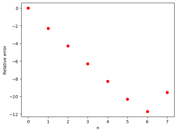
Here’s an example on how you could use Sympy where we compare the symbolic calculation with an integration of a function \(f(x)\) by the Trapezoidal rule. Here we show an example code that evaluates the integral \(\int_0^1 dx x^2 = 1/3\). The following code for the trapezoidal rule allows you to plot the relative error by comparing with the exact result. By increasing to \(10^8\) points one arrives at a region where numerical errors start to accumulate.
%matplotlib inline

from math import log10
import numpy as np
from sympy import Symbol, integrate
import matplotlib.pyplot as plt
# function for the trapezoidal rule
def Trapez(a,b,f,n):
   h = (b-a)/float(n)
   s = 0
   x = a
   for i in range(1,n,1):
       x = x+h
       s = s+ f(x)
   s = 0.5*(f(a)+f(b)) +s
   return h*s
#  function to compute pi
def function(x):
    return x*x
# define integration limits
a = 0.0;  b = 1.0;
# find result from sympy
# define x as a symbol to be used by sympy
x = Symbol('x')
exact = integrate(function(x), (x, a, b))
# set up the arrays for plotting the relative error
n = np.zeros(9); y = np.zeros(9);
# find the relative error as function of integration points
for i in range(1, 8, 1):
    npts = 10**i
    result = Trapez(a,b,function,npts)
    RelativeError = abs((exact-result)/exact)
    n[i] = log10(npts); y[i] = log10(RelativeError);
plt.plot(n,y, 'ro')
plt.xlabel('n')
plt.ylabel('Relative error')
plt.show()
4.4. Energy Conservation
Energy conservation is most convenient as a strategy for addressing problems where time does not appear. For example, a particle goes from position \(x_0\) with speed \(v_0\), to position \(x_f\); what is its new speed? However, it can also be applied to problems where time does appear, such as in solving for the trajectory \(x(t)\), or equivalently \(t(x)\).
Energy is conserved in the case where the potential energy, \(V(\boldsymbol{r})\), depends only on position, and not on time. The force is determined by \(V\),
We say a force is conservative if it satisfies the following conditions:
The force \(\boldsymbol{F}\) acting on an object only depends on the position \(\boldsymbol{r}\), that is \(\boldsymbol{F}=\boldsymbol{F}(\boldsymbol{r})\).
For any two points \(\boldsymbol{r}_1\) and \(\boldsymbol{r}_2\), the work done by the force \(\boldsymbol{F}\) on the displacement between these two points is independent of the path taken.
Finally, the curl of the force is zero \(\boldsymbol{\nabla}\times\boldsymbol{F}=0\).
The energy \(E\) of a given system is defined as the sum of kinetic and potential energies,
We define the potential energy at a point \(\boldsymbol{r}\) as the negative work done from a starting point \(\boldsymbol{r}_0\) to a final point \(\boldsymbol{r}\)
If the potential depends on the path taken between these two points there is no unique potential.
As an example, let us study a classical electron which moves in the \(x\)-direction along a surface. The force from the surface is
The constant \(b\) represents the distance between atoms at the surface of the material, \(F_0\) is a constant and \(x\) is the position of the electron.
This is indeed a conservative force since it depends only on position and its curl is zero, that is \(-\boldsymbol{\nabla}\times \boldsymbol{F}=0\). This means that energy is conserved and the integral over the work done by the force is independent of the path taken.
Using the work-energy theorem we can find the work \(W\) done when moving an electron from a position \(x_0\) to a final position \(x\) through the integral
which results in
Since this is related to the change in kinetic energy we have, with \(v_0\) being the initial velocity at a time \(t_0\),
The potential energy, due to energy conservation is
with \(v\) given by the velocity from above.
We can now, in order to find a more explicit expression for the potential energy at a given value \(x\), define a zero level value for the potential. The potential is defined, using the work-energy theorem, as
and if you recall the definition of the indefinite integral, we can rewrite this as
where \(C\) is an undefined constant. The force is defined as the gradient of the potential, and in that case the undefined constant vanishes. The constant does not affect the force we derive from the potential.
We have then
which results in
We can now define
which gives
We have defined work as the energy resulting from a net force acting on an object (or sseveral objects), that is
If we write out this for each component we have
The work done from an initial position to a final one defines also the difference in potential energies
We can write out the differences in potential energies as
and using the expression the differential of a multi-variable function \(f(x,y,z)\)
we can write the expression for the work done as
Comparing the last equation with
we have
leading to
and
and
or just
And this connection is the one we wanted to show.
4.4.1. Net Energy
The net energy, \(E=V+K\) where \(K\) is the kinetic energy, is then conserved,
The same proof can be written more compactly with vector notation,
Inverting the expression for kinetic energy,
allows one to solve for the one-dimensional trajectory \(x(t)\), by finding \(t(x)\),
Note this would be much more difficult in higher dimensions, because you would have to determine which points, \(x,y,z\), the particles might reach in the trajectory, whereas in one dimension you can typically tell by simply seeing whether the kinetic energy is positive at every point between the old position and the new position.
4.5. The Earth-Sun system
We will now venture into a study of a system which is energy conserving. The aim is to see if we (since it is not possible to solve the general equations analytically) we can develop stable numerical algorithms whose results we can trust!
We solve the equations of motion numerically. We will also compute quantities like the energy numerically.
We start with a simpler case first, the Earth-Sun system in two dimensions only. The gravitational force \(F_G\) on the earth from the sun is
where \(G\) is the gravitational constant,
the mass of Earth,
the mass of the Sun and
is the distance between Earth and the Sun. The latter defines what we call an astronomical unit AU.
From Newton’s second law we have then for the \(x\) direction
and
for the \(y\) direction.
Here we will use that \(x=r\cos{(\theta)}\), \(y=r\sin{(\theta)}\) and
We can rewrite
and
for the \(y\) direction.
We can rewrite these two equations
and
as four first-order coupled differential equations
8 1
< < < ! ! M A T H _ B L O C K
8 2
< < < ! ! M A T H _ B L O C K
8 3
< < < ! ! M A T H _ B L O C K
The four coupled differential equations
8 5
< < < ! ! M A T H _ B L O C K
8 6
< < < ! ! M A T H _ B L O C K
8 7
< < < ! ! M A T H _ B L O C K
can be turned into dimensionless equations or we can introduce astronomical units with \(1\) AU = \(1.5\times 10^{11}\).
Using the equations from circular motion (with \(r =1\mathrm{AU}\))
we have
and using that the velocity of Earth (assuming circular motion) is \(v = 2\pi r/\mathrm{yr}=2\pi\mathrm{AU}/\mathrm{yr}\), we have
The four coupled differential equations can then be discretized using Euler’s method as (with step length \(h\))
9 2
< < < ! ! M A T H _ B L O C K
9 3
< < < ! ! M A T H _ B L O C K
9 4
< < < ! ! M A T H _ B L O C K
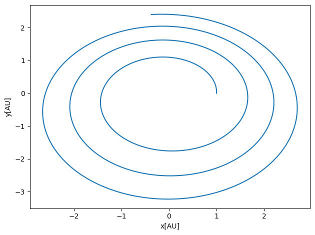
The code here implements Euler’s method for the Earth-Sun system using a more compact way of representing the vectors. Alternatively, you could have spelled out all the variables \(v_x\), \(v_y\), \(x\) and \(y\) as one-dimensional arrays.
# Common imports
import numpy as np
import pandas as pd
from math import *
import matplotlib.pyplot as plt
import os

# Where to save the figures and data files
PROJECT_ROOT_DIR = "Results"
FIGURE_ID = "Results/FigureFiles"
DATA_ID = "DataFiles/"

if not os.path.exists(PROJECT_ROOT_DIR):
    os.mkdir(PROJECT_ROOT_DIR)

if not os.path.exists(FIGURE_ID):
    os.makedirs(FIGURE_ID)

if not os.path.exists(DATA_ID):
    os.makedirs(DATA_ID)

def image_path(fig_id):
    return os.path.join(FIGURE_ID, fig_id)

def data_path(dat_id):
    return os.path.join(DATA_ID, dat_id)

def save_fig(fig_id):
    plt.savefig(image_path(fig_id) + ".png", format='png')


DeltaT = 0.001
#set up arrays
tfinal = 10 # in years
n = ceil(tfinal/DeltaT)
# set up arrays for t, a, v, and x
t = np.zeros(n)
v = np.zeros((n,2))
r = np.zeros((n,2))
# Initial conditions as compact 2-dimensional arrays
r0 = np.array([1.0,0.0])
v0 = np.array([0.0,2*pi])
r[0] = r0
v[0] = v0
Fourpi2 = 4*pi*pi
# Start integrating using Euler's method
for i in range(n-1):
    # Set up the acceleration
    # Here you could have defined your own function for this
    rabs = sqrt(sum(r[i]*r[i]))
    a =  -Fourpi2*r[i]/(rabs**3)
    # update velocity, time and position using Euler's forward method
    v[i+1] = v[i] + DeltaT*a
    r[i+1] = r[i] + DeltaT*v[i]
    t[i+1] = t[i] + DeltaT
# Plot position as function of time
fig, ax = plt.subplots()
#ax.set_xlim(0, tfinal)
ax.set_ylabel('y[AU]')
ax.set_xlabel('x[AU]')
ax.plot(r[:,0], r[:,1])
fig.tight_layout()
save_fig("EarthSunEuler")
plt.show()
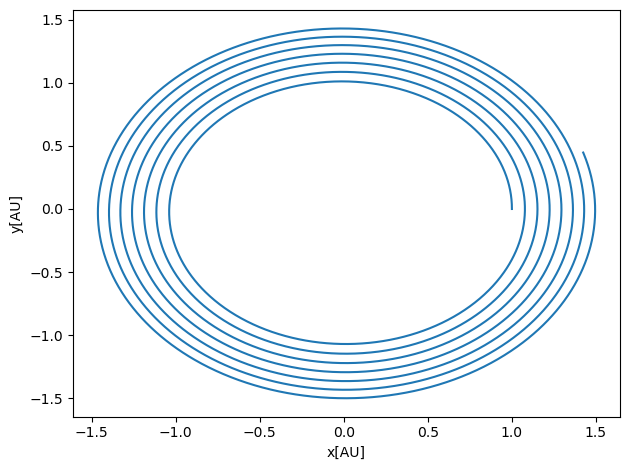
We notice here that Euler’s method doesn’t give a stable orbit. It means that we cannot trust Euler’s method. In a deeper way, as we will see in homework 5, Euler’s method does not conserve energy. It is an example of an integrator which is not symplectic.
Here we present thus two methods, which with simple changes allow us to avoid these pitfalls. The simplest possible extension is the so-called Euler-Cromer method. The changes we need to make to our code are indeed marginal here. We need simply to replace
r[i+1] = r[i] + DeltaT*v[i]
in the above code with the velocity at the new time \(t_{i+1}\)
r[i+1] = r[i] + DeltaT*v[i+1]
By this simple caveat we get stable orbits. Below we derive the Euler-Cromer method as well as one of the most utlized algorithms for sovling the above type of problems, the so-called Velocity-Verlet method.
Let us repeat Euler’s method. We have a differential equation
and if we truncate at the first derivative, we have from the Taylor expansion
which when complemented with \(t_{i+1}=t_i+\Delta t\) forms the algorithm for the well-known Euler method. Note that at every step we make an approximation error of the order of \(O(\Delta t^2)\), however the total error is the sum over all steps \(N=(b-a)/(\Delta t)\) for \(t\in [a,b]\), yielding thus a global error which goes like \(NO(\Delta t^2)\approx O(\Delta t)\).
To make Euler’s method more precise we can obviously decrease \(\Delta t\) (increase \(N\)), but this can lead to loss of numerical precision. Euler’s method is not recommended for precision calculation, although it is handy to use in order to get a first view on how a solution may look like.
Euler’s method is asymmetric in time, since it uses information about the derivative at the beginning of the time interval. This means that we evaluate the position at \(y_1\) using the velocity at \(v_0\). A simple variation is to determine \(x_{n+1}\) using the velocity at \(v_{n+1}\), that is (in a slightly more generalized form)
and
The acceleration \(a_n\) is a function of \(a_n(y_n, v_n, t_n)\) and needs to be evaluated as well. This is the Euler-Cromer method.
4.5.1. Deriving the Velocity-Verlet Method
Let us stay with \(x\) (position) and \(v\) (velocity) as the quantities we are interested in.
We have the Taylor expansion for the position given by
The corresponding expansion for the velocity is
Via Newton’s second law we have normally an analytical expression for the derivative of the velocity, namely
If we add to this the corresponding expansion for the derivative of the velocity
and retain only terms up to the second derivative of the velocity since our error goes as \(O(h^3)\), we have
We can then rewrite the Taylor expansion for the velocity as
Our final equations for the position and the velocity become then
and
Note well that the term \(a_{i+1}\) depends on the position at \(x_{i+1}\). This means that you need to calculate the position at the updated time \(t_{i+1}\) before the computing the next velocity. Note also that the derivative of the velocity at the time \(t_i\) used in the updating of the position can be reused in the calculation of the velocity update as well.
We can now easily add the Verlet method to our original code as
DeltaT = 0.01
#set up arrays
tfinal = 10 # in years
n = ceil(tfinal/DeltaT)
# set up arrays for t, a, v, and x
t = np.zeros(n)
v = np.zeros((n,2))
r = np.zeros((n,2))
# Initial conditions as compact 2-dimensional arrays
r0 = np.array([1.0,0.0])
v0 = np.array([0.0,2*pi])
r[0] = r0
v[0] = v0
Fourpi2 = 4*pi*pi
# Start integrating using the Velocity-Verlet  method
for i in range(n-1):
    # Set up forces, air resistance FD, note now that we need the norm of the vecto
    # Here you could have defined your own function for this
    rabs = sqrt(sum(r[i]*r[i]))
    a =  -Fourpi2*r[i]/(rabs**3)
    # update velocity, time and position using the Velocity-Verlet method
    r[i+1] = r[i] + DeltaT*v[i]+0.5*(DeltaT**2)*a
    rabs = sqrt(sum(r[i+1]*r[i+1]))
    anew = -4*(pi**2)*r[i+1]/(rabs**3)
    v[i+1] = v[i] + 0.5*DeltaT*(a+anew)
    t[i+1] = t[i] + DeltaT
# Plot position as function of time
fig, ax = plt.subplots()
ax.set_ylabel('y[AU]')
ax.set_xlabel('x[AU]')
ax.plot(r[:,0], r[:,1])
fig.tight_layout()
save_fig("EarthSunVV")
plt.show()
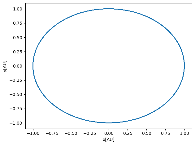
You can easily generalize the calculation of the forces by defining a function which takes in as input the various variables. We leave this as a challenge to you.
4.6. Additional Material: Link between Line Integrals and Conservative forces
The concept of line integrals plays an important role in our discussion of energy conservation, our definition of potentials and conservative forces.
Let us remind ourselves of some the basic elements (most of you may have seen this in a calculus course under the general topic of vector fields).
We define a path integration \(C\), that is we integrate from a point \(\boldsymbol{r}_1\) to a point \(\boldsymbol{r}_2\). Let us assume that the path \(C\) is represented by an arc length \(s\). In three dimension we have the following representation of \(C\)
then our integral of a function \(f(x,y,z)\) along the path \(C\) is defined as
where the initial and final points are \(a\) and \(b\), respectively.
With the definition of a line integral, we can in tunrn set up the theorem of independence of integration path.
Let us define \(f(x,y,z)\), \(g(x,y,z)\) and \(h(x,y,z)\) to be functions which are defined and continuous in a domain \(D\) in space. Then a line integral like the above is said to be independent of path in \(D\), if for every pair of endpoints \(a\) and \(b\) in \(D\) the value of the integral is the same for all paths \(C\) in \(D\) starting from a point \(a\) and ending in a point \(b\). The integral depends thus only on the integration limits and not on the path.
An expression of the form
where \(f\), \(g\) and \(h\) are functions defined in \(D\), is a called a first-order differential form in three variables. The form is said to be exact if it is the differential
of a differentiable function \(u(x,y,z)\) everywhere in \(D\), that is
It is said to be exact if and only if we can then set
and
and
everywhere in the domain \(D\).
In vector language the above means that the differential form
is exact in \(D\) if and only if the vector function (it could be a force, or velocity, acceleration or other vectors we encounter in this course)
is the gradient of a function \(u(x,y,z)\)
If this is the case, we can state the path independence theorem which states that with functions \(f(x,y,z)\), \(g(x,y,z)\) and \(h(x,y,z)\) that fulfill the above exactness conditions, the line integral
is independent of path in \(D\) if and only if the differential form under the integral sign is exact in \(D\).
This is the path independence theorem.
We will not give a proof of the theorem. You can find this in any vector analysis chapter in a mathematics textbook.
We note however that the path integral from a point \(p\) to a final point \(q\) is given by
Assume now that we have a dependence on a variable \(s\) for \(x\), \(y\) and \(z\). We have then
This last equation
is the analogue of the usual formula
with \(F'(x)=f(x)\).
We remember that a the work done by a force \(\boldsymbol{F}=f\boldsymbol{e}_1+g\boldsymbol{e}_2+h\boldsymbol{e}_3\) on a displacemnt \(d\boldsymbol{r}\) is
From the path independence theorem, we know that this has to result in the difference between the two endpoints only. This is exact if and only if the force is the force \(\boldsymbol{F}\) is the gradient of a scalar function \(u\). We call this scalar function, which depends only the positions \(x,y,z\) for the potential energy \(V(x,y,z)=V(\boldsymbol{r})\).
We have thus
and we define this as
Such a force is called a conservative force. The above expression can be used to demonstrate energy conservation.
Finally we can define the criterion for exactness and independence of path. This theorem states that if \(f(x,y,z)\), \(g(x,y,z)\) and \(h(x,y,z)\) are continuous functions with continuous first partial derivatives in the domain \(D\), then the line integral
is independent of path in \(D\) when
and
and
This leads to the curl of \(\boldsymbol{F}\) being zero
A conservative force \(\boldsymbol{F}\) is a defined as the partial derivative of a scalar potential which depends only on the position,
This leads to conservation of energy and a path independent line integral as long as the curl of the force is zero, that is
4.7. Exercises
4.7.1. Exercise: Conservation laws, Energy and momentum
How do we define a conservative force?
A conservative force is a force whose property is that the total work done in moving an object between two points is independent of the taken path. This means that the work on an object under the influence of a conservative force, is independent on the path of the object. It depends only on the spatial degrees of freedom and it is possible to assign a numerical value for the potential at any point. It leads to conservation of energy. The gravitational force is an example of a conservative force.
If you wish to read more about conservative forces or not, Feyman’s lectures from 1963 are quite interesting. He states for example that All fundamental forces in nature appear to be conservative. This statement was made while developing his argument that there are no nonconservative forces. You may enjoy the link to Feynman’s lecture.
An important condition for the final work to be independent of the path is that the curl of the force is zero, that is
Use the work-energy theorem to show that energy is conserved with a conservative force. The work-energy theorem states that the work done \(W\) by a force \(\boldsymbol{F}\) that moves an object from a position \(\boldsymbol{r}_0\) to a new position \(\boldsymbol{r}_1\)
where \(v_1^2\) is the velocity squared at a time \(t_1\) and \(v_0^2\) the corresponding quantity at a time \(t_0\). The work done is thus the difference in kinetic energies. We can rewrite the above equation as
that is the final kinetic energy is equal to the initial kinetic energy plus the work done by the force over a given path from a position \(\boldsymbol{r}_0\) at time \(t_0\) to a final position position \(\boldsymbol{r}_1\) at a later time \(t_1\).
Assume that you have only internal two-body forces acting on \(N\) objects in an isolated system. The force from object \(i\) on object \(j\) is \(\boldsymbol{f}_{ij}\). Show that the linear momentum is conserved.
Here we use Newton’s third law and assume that our system is only affected by so-called internal forces. This means that the force \(\boldsymbol{f}_{ij}\) from object \(i\) acting on object \(j\) is equal to the force acting on object \(j\) from object \(i\) but with opposite sign, that is \(\boldsymbol{f}_{ij}=-\boldsymbol{f}_{ji}\).
The total linear momentum is defined as
where \(i\) runs over all objects, \(m_i\) is the mass of object \(i\) and \(\boldsymbol{v}_i\) its corresponding velocity.
The force acting on object \(i\) from all the other objects is (lower case letters for individual objects and upper case letters for total quantities)
Summing over all objects the net force is
We are summing freely over all objects with the constraint that \(i\ne j\) (no self-interactions). We can now manipulate the double sum as
Convince yourself about this by setting \(N=2\) and \(N=3\). Nweton’s third law says \(\boldsymbol{f}_{ij}=-\boldsymbol{f}_{ji}\), which means we have
The total force due to internal degrees of freedom only is thus \(0\). If we then use the definition that
where we assumed that \(m_i\) is independent of time, we see that time derivative of the total momentum is zero. We say then that the linear momentum is a constant of the motion. It is conserved.
4.7.2. Exercise: Conservation of angular momentum
Define angular momentum and the torque for a single object with external forces only.
The angular moment \(\boldsymbol{l}_i\) for a given object \(i\) is defined as
where \(\boldsymbol{p}_i=m_i\boldsymbol{v}_i\). With external forces only defining the acceleration and the mass being time independent, the momentum is the integral over the external force as function of time, that is
The torque for one object is
Define angular momentum and the torque for a system with \(N\) objects/particles with external and internal forces. The force from object \(i\) on object \(j\) is \(\boldsymbol{F}_{ij}\).
The total angular momentum \(\boldsymbol{L}\) is defined as
and the total torque is (using the expression for one object from 2a)
The force acting on one object is \(\boldsymbol{f}_i=\boldsymbol{f}_i^{\mathrm{ext}}+\sum_{j=1}^N\boldsymbol{f}_{ji}\).
With internal forces only, what is the mathematical form of the forces that allows for angular momentum to be conserved?
Using the results from 1c, we can rewrite without external forces our torque as
which gives
We can rewrite this as (convince yourself again about this)
and using Newton’s third law we have
If the force is proportional to \(\boldsymbol{r}_i -\boldsymbol{r}_j\) then angular momentum is conserved since the cross-product of a vector with itself is zero. We say thus that angular momentum is a constant of the motion.
4.7.3. Exsercise: Example of potential
Consider a particle of mass \(m\) moving according to the potential
Is energy conserved? If so, why?
In this exercise \(A\) and \(a\) are constants. The force is given by the derivative of \(V\) with respect to the spatial degrees of freedom and since the potential depends only on position, the force is conservative and energy is conserved. Furthermore, the curl of the force is zero. To see this we need first to compute the derivatives of the potential with respect to \(x\), \(y\) and \(z\). We have that
and
and
The components of the curl of \(\boldsymbol{F}\) are
and
and
The force is a conservative one.
Which of the quantities, \(p_x,p_y,p_z\) are conserved?
Taking the derivatives with respect to time shows that only \(p_y\) is conserved We see this directly from the above expressions for the force, since the derivative with respect to time of the momentum is simply the force. Thus, only the \(y\)-component of the momentum is conserved, see the expressions above for the forces,
For the next exercise, we also need the following derivatives
and
and
Which of the quantities, \(L_x,L_y,L_z\) are conserved?
Using that \(\boldsymbol{L}=\boldsymbol{r}\times\boldsymbol{p}\) and that
we have that the different components are
and
and
Only \(L_y\) is conserved.
4.7.4. Exercise: forces and potentials
A particle of mass \(m\) has velocity \(v=\alpha/x\), where \(x\) is its displacement.
Find the force \(F(x)\) responsible for the motion.
Here, since the force is assumed to be conservative (only dependence on \(x\)), we can use energy conservation. Assuming that the total energy at \(t=0\) is \(E_0\), we have
Taking the derivative wrt \(x\) we have
and since \(F(x)=-dV/dx\) we have
A particle is thereafter under the influence of a force \(F=-kx+kx^3/\alpha^2\), where \(k\) and \(\alpha\) are constants and \(k\) is positive.
Determine \(V(x)\) and discuss the motion. It can be convenient here to make a sketch/plot of the potential as function of \(x\).
We assume that the potential is zero at say \(x=0\). Integrating the force from zero to \(x\) gives
The following code plots the potential. We have chosen values of \(\alpha=k=1.0\). Feel free to experiment with other values. We plot \(V(x)\) for a domain of \(x\in [-2,2]\).
import numpy as np
import matplotlib.pyplot as plt
import math

x0= -2.0
xn = 2.1
Deltax = 0.1
alpha = 1.0
k = 1.0
#set up arrays
x = np.arange(x0,xn,Deltax)
n = np.size(x)
V = np.zeros(n)
V = 0.5*k*x*x-0.25*k*(x**4)/(alpha*alpha)
plt.plot(x, V)
plt.xlabel("x")
plt.ylabel("V")
plt.show()
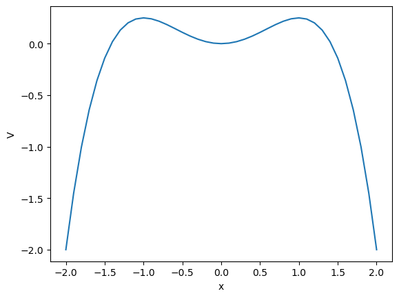
From the plot here (with the chosen parameters)
we see that with a given initial velocity we can overcome the potential energy barrier
and leave the potential well for good.
If the initial velocity is smaller (see next exercise) than a certain value, it will remain trapped in the potential well and oscillate back and forth around \(x=0\). This is where the potential has its minimum value.
If the kinetic energy at \(x=0\) equals the maximum potential energy, the object will oscillate back and forth between the minimum potential energy at \(x=0\) and the turning points where the kinetic energy turns zero. These are the so-called non-equilibrium points.
What happens when the energy of the particle is \(E=(1/4)k\alpha^2\)? Hint: what is the maximum value of the potential energy?
From the figure we see that the potential has a minimum at at \(x=0\) then rises until \(x=\alpha\) before falling off again. The maximum potential, \(V(x\pm \alpha) = k\alpha^2/4\). If the energy is higher, the particle cannot be contained in the well. The turning points are thus defined by \(x=\pm \alpha\). And from the previous plot you can easily see that this is the case (\(\alpha=1\) in the abovementioned Python code).
4.7.5. Exercise: Work-energy theorem and conservation laws
This exercise was partly discussed above. We will study a classical electron which moves in the \(x\)-direction along a surface. The force from the surface is
The constant \(b\) represents the distance between atoms at the surface of the material, \(F_0\) is a constant and \(x\) is the position of the electron.
Is this a conservative force? And if so, what does that imply?
This is indeed a conservative force since it depends only on position and its curl is zero. This means that energy is conserved and the integral over the work done by the force is independent of the path taken.
Use the work-energy theorem to find the velocity \(v(x)\).
Using the work-energy theorem we can find the work \(W\) done when moving an electron from a position \(x_\ 0\) to a final position \(x\) through the integral
which results in
Since this is related to the change in kinetic energy we have, with \(v_0\) being the initial velocity at a time \(t_0\),
With the above expression for the force, find the potential energy.
The potential energy, due to energy conservation is
with \(v\) given by the previous answer. We can now, in order to find a more explicit expression for the potential energy at a given value \(x\), define a zero level value for the potential. The potential is defined , using the work-energy theorem , as
and if you recall the definition of the indefinite integral, we can rewrite this as
where \(C\) is an undefined constant. The force is defined as the gradient of the potential, and in that case the undefined constant vanishes. The constant does not affect the force we derive from the potential.
We have then
which results in
We can now define
which gives
Make a plot of the potential energy and discuss the equilibrium points where the force on the electron is zero. Discuss the physical interpretation of stable and unstable equilibrium points. Use energy conservation.
The following Python code plots the potential
import numpy as np
import pandas as pd
from math import *
import matplotlib.pyplot as plt
Deltax = 0.01
#set up arrays
xinitial = -2.0
xfinal = 2.0
n = ceil((xfinal-xinitial)/Deltax)
x = np.zeros(n)
for i in range(n):
    x[i] = xinitial+i*Deltax
V = np.zeros(n)
# Setting values for the constants.
F0 = 1.0; b = 1.0;
# Defining the potential
V = F0*b/(2*pi)*np.cos(2*pi*x/b)
# Plot position as function of time
fig, ax = plt.subplots()
ax.set_ylabel('V')
ax.set_xlabel('x')
ax.plot(x, V)
fig.tight_layout()
plt.show()
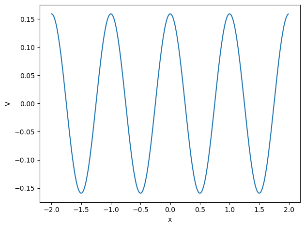
We have stable equilibrium points for every minimum of the \(\cos\) function and unstable equilibrium points where it has its maximimum values. At the minimum the particle has the lowest potential energy and the largest kinetic energy whereas at the maxima it has the largest potential energy and lowest kinetic energy.
4.7.6. Exsercise: Rocket, Momentum and mass
Taylor exercise 3.11.
Consider the rocket of mass \(M\) moving with velocity \(v\). After a brief instant, the velocity of the rocket is \(v+\Delta v\) and the mass is \(M-\Delta M\). Momentum conservation gives
In the second step we ignored the term \(\Delta M\Delta v\) since we assume it is small. The last equation gives
Here we let \(\Delta v\rightarrow dv\) and \(\Delta M\rightarrow dM\). We have also assumed that \(M(t) = M_0-kt\). Integrating the expression with lower limits \(v_0=0\) and \(M_0\), one finds
We have ignored gravity here. If we add gravity as the external force, we get when integrating an additional terms \(-gt\), that is
Inserting numbers \(v_e=3000\) m/s, \(M_0/M=2\) and \(g=9.8\) m/s\(^{2}\), we find \(v=900\) m/s. With \(g=0\) the corresponding number is \(2100\) m/s, so gravity reduces the speed acquired in the first two minutes to a little less than half its weight-free value.
If the thrust \(\Delta Mv_e\) is less than the weight \(mg\), the rocket will just sit on the ground until it has shed enough mass that the thrust can overcome the weight, definitely not a good design.
4.7.7. Exercise: More Rockets
This is a continuation of the previous exercise and most of the relevant background material can be found in Taylor chapter 3.2.
Taking the velocity from the previous exercise and integrating over time we find the height
which gives
To do the integral over time we recall that \(M(t')=M_0-\Delta M t'\). We assumed that \(\Delta M=k\) is a constant. We use that \(M_0-M=kt\) and assume that mass decreases by a constant \(k\) times time \(t\).
We obtain then that the integral gives
and defining the variable \(u=M_0-kt'\), with \(du=-kdt'\) and the new limits \(M_0\) when \(t=0\) and \(M_0-kt\) when time is equal to \(t\), we have
and writing out we obtain
Mulitplying with \(-v_e\) we have
which we can rewrite as, using \(M_0=M+kt\),
Inserting into \(y(t)\) we obtain then
Using the numbers from the previous exercise with \(t=2\) min we obtain that \(y\approx 40\) km.
For exercise 3.14 (5pt) we have the equation of motion which reads \(Ma=kv_e-bv\) or
We have that \(dM/dt =-k\) (assumed a constant rate for mass change). We can then replace \(dt\) by \(-dM/k\) and we have
Integrating gives
4.7.8. Exercise: Center of mass
Taylor exercise 3.20. Here Taylor’s chapter 3.3 can be of use. This relation will turn out to be very useful when we discuss systems of many classical particles.
The definition of the center of mass for \(N\) objects can be written as
where \(m_i\) and \(\boldsymbol{r}_i\) are the masses and positions of object \(i\), respectively.
Assume now that we have a collection of \(N_1\) objects with masses \(m_{1i}\) and positions \(\boldsymbol{r}_{1i}\) with \(i=1,\dots,N_1\) and a collection of \(N_2\) objects with masses \(m_{2j}\) and positions \(\boldsymbol{r}_{2j}\) with \(j=1,\dots,N_2\).
The total mass of the two-body system is \(M=M_1+M_2=\sum_{i=1}^{N_1}m_{1i}+\sum_{j=1}^{N_2}m_{2j}\). The center of mass position \(\boldsymbol{R}\) of the whole system satisfies then
where \(\boldsymbol{R}_1\) and \(\boldsymbol{R}_2\) are the the center of mass positions of the two separate bodies and the second equality follows from our rewritten definition of the center of mass applied to each body separately. This is the required result.
4.7.9. Exercise: The Earth-Sun problem
We start with the Earth-Sun system in two dimensions only. The gravitational force \(F_G\) on the earth from the sun is
where \(G\) is the gravitational constant,
the mass of Earth,
the mass of the Sun and
is the distance between Earth and the Sun. The latter defines what we call an astronomical unit AU. From Newton’s second law we have then for the \(x\) direction
and
for the \(y\) direction.
Here we will use that \(x=r\cos{(\theta)}\), \(y=r\sin{(\theta)}\) and
We can rewrite these equations
and
as four first-order coupled differential equations
and
and
and
The four coupled differential equations
and
and
and
can be turned into dimensionless equations or we can introduce astronomical units with \(1\) AU = \(1.5\times 10^{11}\).
Using the equations from circular motion (with \(r =1\mathrm{AU}\))
we have
and using that the velocity of Earth (assuming circular motion) is \(v = 2\pi r/\mathrm{yr}=2\pi\mathrm{AU}/\mathrm{yr}\), we have
The four coupled differential equations can then be discretized using Euler’s method as (with step length \(h\))
and
and
and
The code here implements Euler’s method for the Earth-Sun system using a more compact way of representing the vectors. Alternatively, you could have spelled out all the variables \(v_x\), \(v_y\), \(x\) and \(y\) as one-dimensional arrays.
# Common imports
import numpy as np
import pandas as pd
from math import *
import matplotlib.pyplot as plt
import os

# Where to save the figures and data files
PROJECT_ROOT_DIR = "Results"
FIGURE_ID = "Results/FigureFiles"
DATA_ID = "DataFiles/"

if not os.path.exists(PROJECT_ROOT_DIR):
    os.mkdir(PROJECT_ROOT_DIR)

if not os.path.exists(FIGURE_ID):
    os.makedirs(FIGURE_ID)

if not os.path.exists(DATA_ID):
    os.makedirs(DATA_ID)

def image_path(fig_id):
    return os.path.join(FIGURE_ID, fig_id)

def data_path(dat_id):
    return os.path.join(DATA_ID, dat_id)

def save_fig(fig_id):
    plt.savefig(image_path(fig_id) + ".png", format='png')


DeltaT = 0.01
#set up arrays
tfinal = 10 # in years
n = ceil(tfinal/DeltaT)
# set up arrays for t, a, v, and x
t = np.zeros(n)
v = np.zeros((n,2))
r = np.zeros((n,2))
# Initial conditions as compact 2-dimensional arrays
r0 = np.array([1.0,0.0])
v0 = np.array([0.0,2*pi])
r[0] = r0
v[0] = v0
Fourpi2 = 4*pi*pi
# Start integrating using Euler's method
for i in range(n-1):
    # Set up the acceleration
    # Here you could have defined your own function for this
    rabs = sqrt(sum(r[i]*r[i]))
    a =  -Fourpi2*r[i]/(rabs**3)
    # update velocity, time and position using Euler's forward method
    v[i+1] = v[i] + DeltaT*a
    r[i+1] = r[i] + DeltaT*v[i]
    t[i+1] = t[i] + DeltaT
# Plot position as function of time
fig, ax = plt.subplots()
#ax.set_xlim(0, tfinal)
ax.set_xlabel('x[AU]')
ax.set_ylabel('y[AU]')
ax.plot(r[:,0], r[:,1])
fig.tight_layout()
save_fig("EarthSunEuler")
plt.show()
We notice here that Euler’s method doesn’t give a stable orbit with for example \(\Delta t =0.01\). It means that we cannot trust Euler’s method. Euler’s method does not conserve energy. It is an example of an integrator which is not symplectic.
Here we present thus two methods, which with simple changes allow us to avoid these pitfalls. The simplest possible extension is the so-called Euler-Cromer method. The changes we need to make to our code are indeed marginal here. We need simply to replace
r[i+1] = r[i] + DeltaT*v[i]
in the above code with the velocity at the new time \(t_{i+1}\)
r[i+1] = r[i] + DeltaT*v[i+1]
By this simple caveat we get stable orbits. Below we derive the Euler-Cromer method as well as one of the most utlized algorithms for solving the above type of problems, the so-called Velocity-Verlet method.
Let us repeat Euler’s method. We have a differential equation
and if we truncate at the first derivative, we have from the Taylor expansion
which when complemented with \(t_{i+1}=t_i+\Delta t\) forms the algorithm for the well-known Euler method. Note that at every step we make an approximation error of the order of \(O(\Delta t^2)\), however the total error is the sum over all steps \(N=(b-a)/(\Delta t)\) for \(t\in [a,b]\), yielding thus a global error which goes like \(NO(\Delta t^2)\approx O(\Delta t)\).
To make Euler’s method more precise we can obviously decrease \(\Delta t\) (increase \(N\)), but this can lead to loss of numerical precision. Euler’s method is not recommended for precision calculation, although it is handy to use in order to get a first view on how a solution may look like.
Euler’s method is asymmetric in time, since it uses information about the derivative at the beginning of the time interval. This means that we evaluate the position at \(y_1\) using the velocity at \(v_0\). A simple variation is to determine \(x_{n+1}\) using the velocity at \(v_{n+1}\), that is (in a slightly more generalized form)
and
The acceleration \(a_n\) is a function of \(a_n(y_n, v_n, t_n)\) and needs to be evaluated as well. This is the Euler-Cromer method. It is easy to change the above code and see that with the same time step we get stable results.
Let us stay with \(x\) (position) and \(v\) (velocity) as the quantities we are interested in.
We have the Taylor expansion for the position given by
The corresponding expansion for the velocity is
Via Newton’s second law we have normally an analytical expression for the derivative of the velocity, namely
If we add to this the corresponding expansion for the derivative of the velocity
and retain only terms up to the second derivative of the velocity since our error goes as \(O(h^3)\), we have
We can then rewrite the Taylor expansion for the velocity as
Our final equations for the position and the velocity become then
and
Note well that the term \(a_{i+1}\) depends on the position at \(x_{i+1}\). This means that you need to calculate the position at the updated time \(t_{i+1}\) before the computing the next velocity. Note also that the derivative of the velocity at the time \(t_i\) used in the updating of the position can be reused in the calculation of the velocity update as well.
We can now easily add the Verlet method to our original code as
DeltaT = 0.01
#set up arrays
tfinal = 10
n = ceil(tfinal/DeltaT)
# set up arrays for t, a, v, and x
t = np.zeros(n)
v = np.zeros((n,2))
r = np.zeros((n,2))
# Initial conditions as compact 2-dimensional arrays
r0 = np.array([1.0,0.0])
v0 = np.array([0.0,2*pi])
r[0] = r0
v[0] = v0
Fourpi2 = 4*pi*pi
# Start integrating using the Velocity-Verlet  method
for i in range(n-1):
    # Set up forces, air resistance FD, note now that we need the norm of the vecto
    # Here you could have defined your own function for this
    rabs = sqrt(sum(r[i]*r[i]))
    a =  -Fourpi2*r[i]/(rabs**3)
    # update velocity, time and position using the Velocity-Verlet method
    r[i+1] = r[i] + DeltaT*v[i]+0.5*(DeltaT**2)*a
    rabs = sqrt(sum(r[i+1]*r[i+1]))
    anew = -4*(pi**2)*r[i+1]/(rabs**3)
    v[i+1] = v[i] + 0.5*DeltaT*(a+anew)
    t[i+1] = t[i] + DeltaT
# Plot position as function of time
fig, ax = plt.subplots()
ax.set_xlabel('x[AU]')
ax.set_ylabel('y[AU]')
ax.plot(r[:,0], r[:,1])
fig.tight_layout()
save_fig("EarthSunVV")
plt.show()

You can easily generalize the calculation of the forces by defining a function which takes in as input the various variables. We leave this as a challenge to you.
Running the above code for various time steps we see that the Velocity-Verlet is fully stable for various time steps.
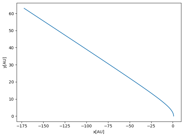
We can also play around with different initial conditions in order to find the escape velocity from an orbit around the sun with distance one astronomical unit, 1 AU. The theoretical value for the escape velocity, is given by
and with \(r=1\) AU, this means that the escape velocity is \(2\pi\sqrt{2}\) AU/yr. To obtain this we required that the kinetic energy of Earth equals the potential energy given by the gravitational force.
Setting
and with \(GM_{\odot}=4\pi^2\) we obtain the above relation for the velocity. Setting an initial velocity say equal to \(9\) in the above code, yields a planet (Earth) which escapes a stable orbit around the sun, as seen by running the code here.
DeltaT = 0.01
#set up arrays
tfinal = 100
n = ceil(tfinal/DeltaT)
# set up arrays for t, a, v, and x
t = np.zeros(n)
v = np.zeros((n,2))
r = np.zeros((n,2))
# Initial conditions as compact 2-dimensional arrays
r0 = np.array([1.0,0.0])
# setting initial velocity larger than escape velocity
v0 = np.array([0.0,9.0])
r[0] = r0
v[0] = v0
Fourpi2 = 4*pi*pi
# Start integrating using the Velocity-Verlet  method
for i in range(n-1):
    # Set up forces, air resistance FD, note now that we need the norm of the vecto
    # Here you could have defined your own function for this
    rabs = sqrt(sum(r[i]*r[i]))
    a =  -Fourpi2*r[i]/(rabs**3)
    # update velocity, time and position using the Velocity-Verlet method
    r[i+1] = r[i] + DeltaT*v[i]+0.5*(DeltaT**2)*a
    rabs = sqrt(sum(r[i+1]*r[i+1]))
    anew = -4*(pi**2)*r[i+1]/(rabs**3)
    v[i+1] = v[i] + 0.5*DeltaT*(a+anew)
    t[i+1] = t[i] + DeltaT
# Plot position as function of time
fig, ax = plt.subplots()
ax.set_xlabel('x[AU]')
ax.set_ylabel('y[AU]')
ax.plot(r[:,0], r[:,1])
fig.tight_layout()
save_fig("EscapeEarthSunVV")
plt.show()
4.7.10. Exercise Conservative forces
Which of the following force are conservative? All three forces depend only on \(\boldsymbol{r}\) and satisfy the first condition for being conservative.
\(\boldsymbol{F}=k(x\boldsymbol{i}+2y\boldsymbol{j}+3z\boldsymbol{k})\) where \(k\) is a constant.
The curl is zero and the force is conservative. The potential energy is upon integration \(V(x)=-k(1/2x^2+y^2+3/2z^2)\). Taking the derivative shows that this is indeed the case since it gives back the force.
\(\boldsymbol{F}=y\boldsymbol{i}+x\boldsymbol{j}+0\boldsymbol{k}\).
This force is also conservative since it depends only on the coordinates and its curl is zero. To find the potential energy, since the integral is path independent, we can choose to integrate along any direction. The simplest is start from \(x=0\) as origin and follow a path along the \(x\)-axis (which gives zero) and then parallel to the \(y\)-axis, which results in \(V(x,y) = -xy\). Taking the derivative with respect to \(x\) and \(y\) gives us back the expression for the force.
\(\boldsymbol{F}=k(-y\boldsymbol{i}+x\boldsymbol{j}+0\boldsymbol{k})\) where \(k\) is a constant.
Here the curl is \((0,0,2)\) and the force is not conservative.
2d For those which are conservative, find the corresponding potential energy \(V\) and verify that direct differentiation that \(\boldsymbol{F}=-\boldsymbol{\nabla} V\).
See the answers to each exercise above.
4.7.11. Exercise: The Lennard-Jones potential
The Lennard-Jones potential is often used to describe the interaction between two atoms or ions or molecules. If you end up doing materals science and molecular dynamics calculations, it is very likely that you will encounter this potential model. The expression for the potential energy is
where \(V_0\), \(a\) and \(b\) are constants and the potential depends only on the relative distance between two objects \(i\) and \(j\), that is \(r=\vert\vert\boldsymbol{r}_i-\boldsymbol{r}_j\vert\vert=\sqrt{(x_i-x_j)^2+(y_i-y_j)^2+(z_i-z_j)^2}\).
Sketch/plot the potential (choose some values for the constants in doing so).
The following Python code plots the potential
# Common imports
import numpy as np
from math import *
import matplotlib.pyplot as plt

Deltar = 0.01
#set up arrays
rinitial = 1.8
rfinal = 3.
n = ceil((rfinal-rinitial)/Deltar)
r = np.zeros(n)
for i in range(n):
    r[i] = rinitial+i*Deltar
V = np.zeros(n)
# Initial conditions as compact 2-dimensional arrays
a = 2.0
b = 2.0
V0 = 10.0
V = V0*((a/r)**(12)-(b/r)**6)
# Plot position as function of time
fig, ax = plt.subplots()
#ax.set_xlim(0, tfinal)
ax.set_ylabel('V')
ax.set_xlabel('r')
ax.plot(r, V)
fig.tight_layout()
plt.show()
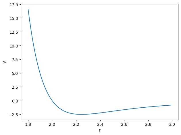
Find and classify the equilibrium points.
Here there is only one equilibrium point when we take the derivative of the potential with respect to the relative distance.
The derivative with respect to \(r\), the relative distance, is
and this is zero when
If we choose \(a=2\) and \(b=2\) then \(r=2\times 2^{1/6}\). Since the second derivative is positive for all \(r\) for our choices of \(a\) and \(b\) (convince yourself about this), then this value of \(r\) has to correspond to a minimum of the potential. This agrees with our graph from the figure above (run the code to produce the figure).
What is the force acting on one of the objects (an atom for example) from the other object? Is this a conservative force?
From the previous exercise we have
We need the gradient and since the force on particle \(i\) is given by \(\boldsymbol{F}_i=\boldsymbol{\nabla}_i V(\boldsymbol{r}_i-\boldsymbol{r}_j)\), we obtain
Here \(r = \vert\vert \boldsymbol{r}_i-\boldsymbol{r}_j\vert \vert\). If we have more than two particles, we need to sum over all other particles \(j\). We have thus to introduce a sum over all particles \(N\). The force on particle \(i\) at position \(\boldsymbol{r}_i\) from all particles \(j\) at their positions \(\boldsymbol{r}_j\) results in the equation of motion (note that we have divided by the mass \(m\) here)
This is also a conservative force, with zero curl as well.
4.7.12. Exercise: particle in a new potential
Consider a particle of mass \(m\) moving in a one-dimensional potential,
Plot the potential and discuss eventual equilibrium points. Is this a conservative force?
The following Python code gives a plot of potential
# Common imports
import numpy as np
from math import *
import matplotlib.pyplot as plt

Deltax = 0.01
#set up arrays
xinitial = -2.0
xfinal = 2.0
n = ceil((xfinal-xinitial)/Deltax)
x = np.zeros(n)
for i in range(n):
    x[i] = xinitial+i*Deltax
V = np.zeros(n)
# Initial conditions as compact 2-dimensional arrays
alpha = 0.81
beta = 0.5
print(sqrt(alpha/beta))
V = -alpha*x*x*0.5 + beta*(x**4)*0.25
# Plot position as function of time
fig, ax = plt.subplots()
#ax.set_xlim(0, tfinal)
ax.set_xlabel('x')
ax.set_ylabel('V[s]')
ax.plot(x, V)
fig.tight_layout()
plt.show()
1.2727922061357855
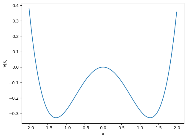
Here we have chosen \(\alpha=0.81\) and \(\beta=0.5\). Taking the derivative of \(V\) with respect to \(x\) gives two minima (and it is easy to see here that the second derivative is positive) at \(x\pm\sqrt{\alpha/\beta}\) and a maximum at \(x=0\). The derivative is
which gives when we require that it should equal zero the above values. As we can see from the plot (run the above Python code), we have two so-called stable equilibrium points (where the potential has its minima) and an unstable equilibrium point.
The force is conservative since it depends only on \(x\) and has a curl which is zero.
Compute the second derivative of the potential and find its miminum position(s). Using the Taylor expansion of the potential around its minimum (see Taylor section 5.1) to define a spring constant \(k\). Use the spring constant to find the natural (angular) frequency \(\omega_0=\sqrt{k/m}\). We call the new spring constant for an effective spring constant.
In the solution to the previous exercise we listed the values where the derivatives of the potential are zero. Taking the second derivatives we have that
and for \(\alpha,\beta > 0\) (we assume they are positive constants) we see that when \(x=0\) that the the second derivative is negative, which means this is a maximum. For \(x=\pm\sqrt{\alpha/\beta}\) we see that the second derivative is positive. Thus these points correspond to two minima.
Assume now we Taylor-expand the potential around one of these minima, say \(x_{\mathrm{min}}=\sqrt{\alpha/\beta}\). We have thus
Since we are at point where the first derivative is zero and inserting the value for the second derivative of \(V\), keeping only terms up to the second derivative and finally taking the derivative with respect to \(x\), we find the expression for the force
and setting in the expression for the second derivative at the minimum we find
Thus our effective spring constant \(k=2\alpha\).
We ignore the second term in the potential energy and keep only the term proportional to the effective spring constant, that is a force \(F\propto kx\). Find the acceleration and set up the differential equation. Find the general analytical solution for these harmonic oscillations. You don’t need to find the constants in the general solution.
Here we simplify our force by rescaling our zeroth point so that we have a force (setting \(x_{\mathrm{min}}=0\))
with \(k=2\alpha\). Defining a natural frequency \(\omega_0 = \sqrt{k/m}\), where \(m\) is the mass of our particle, we have the following equation of motion
which has as analytical solution \(x(t)=A\cos{(\omega_0t)}+B\sin{(\omega_0t)}\) and velocity \(x(t)=-\omega_0A\sin{(\omega_0t)}+\omega_0B\cos{(\omega_0t)}\). The initial conditions are used to define \(A\) and \(B\).
4.7.13. Exercise: Testing Energy conservation
The code here implements Euler’s method for the Earth-Sun system using a more compact way of representing the vectors. Alternatively, you could have spelled out all the variables \(v_x\), \(v_y\), \(x\) and \(y\) as one-dimensional arrays. It tests conservation of potential and kinetic energy as functions of time, in addition to the total energy, again as function of time
Note: in all codes we have used scaled equations so that the gravitational constant times the mass of the sum is given by \(4\pi^2\) and the mass of the earth is set to one in the calculations of kinetic and potential energies. Else, we would get very large results.
# Common imports
import numpy as np
import pandas as pd
from math import *
import matplotlib.pyplot as plt
import os

# Where to save the figures and data files
PROJECT_ROOT_DIR = "Results"
FIGURE_ID = "Results/FigureFiles"
DATA_ID = "DataFiles/"

if not os.path.exists(PROJECT_ROOT_DIR):
    os.mkdir(PROJECT_ROOT_DIR)

if not os.path.exists(FIGURE_ID):
    os.makedirs(FIGURE_ID)

if not os.path.exists(DATA_ID):
    os.makedirs(DATA_ID)

def image_path(fig_id):
    return os.path.join(FIGURE_ID, fig_id)

def data_path(dat_id):
    return os.path.join(DATA_ID, dat_id)

def save_fig(fig_id):
    plt.savefig(image_path(fig_id) + ".png", format='png')

# Initial values, time step, positions and velocites

DeltaT = 0.0001
#set up arrays
tfinal = 100 # in years
n = ceil(tfinal/DeltaT)
# set up arrays for t, a, v, and x
t = np.zeros(n)
v = np.zeros((n,2))
r = np.zeros((n,2))

# setting up the kinetic, potential and total energy, note only functions of time
EKinetic = np.zeros(n)
EPotential = np.zeros(n)
ETotal = np.zeros(n)

# Initial conditions as compact 2-dimensional arrays


r0 = np.array([1.0,0.0])
v0 = np.array([0.0,2*pi])
r[0] = r0
v[0] = v0
Fourpi2 = 4*pi*pi
# Setting up variables for the calculation of energies
#  distance that defines rabs in potential energy
rabs0 = sqrt(sum(r[0]*r[0]))
#  Initial kinetic energy. Note that we skip the mass of the Earth here, that is MassEarth=1 in all codes
EKinetic[0] = 0.5*sum(v0*v0)
#  Initial potential energy  (note negative sign, why?)
EPotential[0] = -4*pi*pi/rabs0
#  Initial total energy
ETotal[0] = EPotential[0]+EKinetic[0]
# Start integrating using Euler's method
for i in range(n-1):
    # Set up the acceleration
    # Here you could have defined your own function for this
    rabs = sqrt(sum(r[i]*r[i]))
    a =  -Fourpi2*r[i]/(rabs**3)
    # update Energies, velocity, time and position using Euler's forward method
    v[i+1] = v[i] + DeltaT*a
    r[i+1] = r[i] + DeltaT*v[i]
    t[i+1] = t[i] + DeltaT
    EKinetic[i+1] = 0.5*sum(v[i+1]*v[i+1])
    EPotential[i+1] = -4*pi*pi/sqrt(sum(r[i+1]*r[i+1]))
    ETotal[i+1] = EPotential[i+1]+EKinetic[i+1]
# Plot energies as functions of time

fig, axs = plt.subplots(3, 1)
axs[0].plot(t, EKinetic)
axs[0].set_xlim(0, tfinal)
axs[0].set_ylabel('Kinetic energy')
axs[1].plot(t, EPotential)
axs[1].set_ylabel('Potential Energy')
axs[2].plot(t, ETotal)
axs[2].set_xlabel('Time [yr]')
axs[2].set_ylabel('Total Energy')
fig.tight_layout()
save_fig("EarthSunEuler")
plt.show()
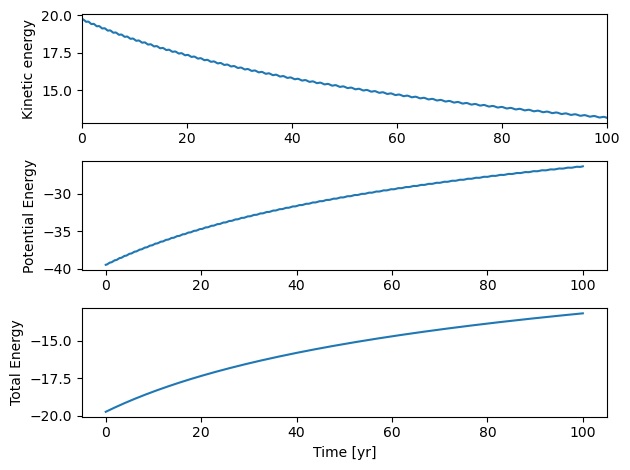
We see very clearly that Euler’s method does not conserve energy!! Try to reduce the time step \(\Delta t\). What do you see?
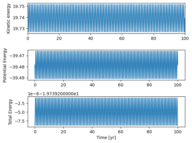
With the Euler-Cromer method, the only thing we need is to update the position at a time \(t+1\) with the update velocity from the same time. Thus, the change in the code is extremely simply, and energy is suddenly conserved. Note that the error runs like \(O(\Delta t)\) and this is why we see the larger oscillations. But within this oscillating energy envelope, we see that the energies swing between a max and a min value and never exceed these values.
# Common imports
import numpy as np
import pandas as pd
from math import *
import matplotlib.pyplot as plt
import os

# Where to save the figures and data files
PROJECT_ROOT_DIR = "Results"
FIGURE_ID = "Results/FigureFiles"
DATA_ID = "DataFiles/"

if not os.path.exists(PROJECT_ROOT_DIR):
    os.mkdir(PROJECT_ROOT_DIR)

if not os.path.exists(FIGURE_ID):
    os.makedirs(FIGURE_ID)

if not os.path.exists(DATA_ID):
    os.makedirs(DATA_ID)

def image_path(fig_id):
    return os.path.join(FIGURE_ID, fig_id)

def data_path(dat_id):
    return os.path.join(DATA_ID, dat_id)

def save_fig(fig_id):
    plt.savefig(image_path(fig_id) + ".png", format='png')

# Initial values, time step, positions and velocites

DeltaT = 0.0001
#set up arrays
tfinal = 100 # in years
n = ceil(tfinal/DeltaT)
# set up arrays for t, a, v, and x
t = np.zeros(n)
v = np.zeros((n,2))
r = np.zeros((n,2))

# setting up the kinetic, potential and total energy, note only functions of time
EKinetic = np.zeros(n)
EPotential = np.zeros(n)
ETotal = np.zeros(n)

# Initial conditions as compact 2-dimensional arrays


r0 = np.array([1.0,0.0])
v0 = np.array([0.0,2*pi])
r[0] = r0
v[0] = v0
Fourpi2 = 4*pi*pi
# Setting up variables for the calculation of energies
#  distance that defines rabs in potential energy
rabs0 = sqrt(sum(r[0]*r[0]))
#  Initial kinetic energy. Note that we skip the mass of the Earth here, that is MassEarth=1 in all codes
EKinetic[0] = 0.5*sum(v0*v0)
#  Initial potential energy
EPotential[0] = -4*pi*pi/rabs0
#  Initial total energy
ETotal[0] = EPotential[0]+EKinetic[0]
# Start integrating using Euler's method
for i in range(n-1):
    # Set up the acceleration
    # Here you could have defined your own function for this
    rabs = sqrt(sum(r[i]*r[i]))
    a =  -Fourpi2*r[i]/(rabs**3)
    # update velocity, time and position using Euler's forward method
    v[i+1] = v[i] + DeltaT*a
#   Only change when we add the Euler-Cromer method
    r[i+1] = r[i] + DeltaT*v[i+1]
    t[i+1] = t[i] + DeltaT
    EKinetic[i+1] = 0.5*sum(v[i+1]*v[i+1])
    EPotential[i+1] = -4*pi*pi/sqrt(sum(r[i+1]*r[i+1]))
    ETotal[i+1] = EPotential[i+1]+EKinetic[i+1]
# Plot energies as functions of time

fig, axs = plt.subplots(3, 1)
axs[0].plot(t, EKinetic)
axs[0].set_xlim(0, tfinal)
axs[0].set_ylabel('Kinetic energy')
axs[1].plot(t, EPotential)
axs[1].set_ylabel('Potential Energy')
axs[2].plot(t, ETotal)
axs[2].set_xlabel('Time [yr]')
axs[2].set_ylabel('Total Energy')
fig.tight_layout()
save_fig("EarthSunEulerCromer")
plt.show()
Our final equations for the position and the velocity become then
and
Note well that the term \(a_{i+1}\) depends on the position at \(x_{i+1}\). This means that you need to calculate the position at the updated time \(t_{i+1}\) before the computing the next velocity. Note also that the derivative of the velocity at the time \(t_i\) used in the updating of the position can be reused in the calculation of the velocity update as well.
We can now easily add the Verlet method to our original code as
DeltaT = 0.001
#set up arrays
tfinal = 100
n = ceil(tfinal/DeltaT)
# set up arrays for t, a, v, and x
t = np.zeros(n)
v = np.zeros((n,2))
r = np.zeros((n,2))
# Initial conditions as compact 2-dimensional arrays
r0 = np.array([1.0,0.0])
v0 = np.array([0.0,2*pi])
r[0] = r0
v[0] = v0
Fourpi2 = 4*pi*pi

# setting up the kinetic, potential and total energy, note only functions of time
EKinetic = np.zeros(n)
EPotential = np.zeros(n)
ETotal = np.zeros(n)

# Setting up variables for the calculation of energies
#  distance that defines rabs in potential energy
rabs0 = sqrt(sum(r[0]*r[0]))
#  Initial kinetic energy. Note that we skip the mass of the Earth here, that is MassEarth=1 in all codes
EKinetic[0] = 0.5*sum(v0*v0)
#  Initial potential energy
EPotential[0] = -4*pi*pi/rabs0
#  Initial total energy
ETotal[0] = EPotential[0]+EKinetic[0]

# Start integrating using the Velocity-Verlet  method
for i in range(n-1):
    # Set up forces, air resistance FD, note now that we need the norm of the vecto
    # Here you could have defined your own function for this
    rabs = sqrt(sum(r[i]*r[i]))
    a =  -Fourpi2*r[i]/(rabs**3)
    # update velocity, time and position using the Velocity-Verlet method
    r[i+1] = r[i] + DeltaT*v[i]+0.5*(DeltaT**2)*a
    rabs = sqrt(sum(r[i+1]*r[i+1]))
    anew = -4*(pi**2)*r[i+1]/(rabs**3)
    v[i+1] = v[i] + 0.5*DeltaT*(a+anew)
    t[i+1] = t[i] + DeltaT
    EKinetic[i+1] = 0.5*sum(v[i+1]*v[i+1])
    EPotential[i+1] = -4*pi*pi/sqrt(sum(r[i+1]*r[i+1]))
    ETotal[i+1] = EPotential[i+1]+EKinetic[i+1]
# Plot energies as functions of time

fig, axs = plt.subplots(3, 1)
axs[0].plot(t, EKinetic)
axs[0].set_xlim(0, tfinal)
axs[0].set_ylabel('Kinetic energy')
axs[1].plot(t, EPotential)
axs[1].set_ylabel('Potential Energy')
axs[2].plot(t, ETotal)
axs[2].set_xlabel('Time [yr]')
axs[2].set_ylabel('Total Energy')
fig.tight_layout()
save_fig("EarthSunVelocityVerlet")
plt.show()
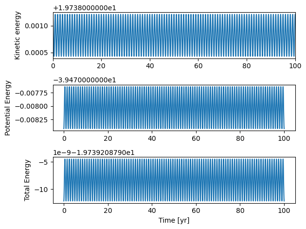
And we see that due to the smaller truncation error that energy conservation is improved as a function of time. Try out different time steps \(\Delta t\) and see if the results improve or worsen.