Let us quickly remind ourselves about the definition of a so-called inertial frame of reference. An inertial frame of reference in classical physics (and in special relativity as well) possesses the property that in this frame of reference a body with zero net force acting upon it does not accelerate; that is, such a body is at rest or moving at a constant velocity. If we recall the definition of Newton's first law, this is essentially its description.
An inertial frame of reference can be defined in analytical terms as a frame of reference that describes time and space homogeneously, isotropically, and in a time-independent manner.
Conceptually, the physics of a system in an inertial frame has no causes external to the system. An inertial frame of reference may also be called an inertial reference frame, inertial frame, Galilean reference frame, or inertial space.
All inertial frames are in a state of constant, rectilinear motion with respect to one another; an accelerometer moving with any of them would detect zero acceleration. Measurements in one inertial frame can be converted to measurements in another by a simple transformation (the Galilean transformation in Newtonian physics and the Lorentz transformation in special relativity). In general relativity, in any region small enough for the curvature of spacetime and tidal forces to be negligible, one can find a set of inertial frames that approximately describe that region.
In a non-inertial reference frame in classical physics and special relativity, the physics of a system vary depending on the acceleration of that frame with respect to an inertial frame, and the usual physical forces must be supplemented by fictitious forces. In contrast, systems in general relativity don't have external causes, because of the principle of geodesic motion.
In classical physics, for example, a ball dropped towards the ground does not go exactly straight down because the Earth is rotating, which means the frame of reference of an observer on Earth is not inertial. The physics must account for the Coriolis effect—in this case thought of as a force—to predict the horizontal motion. Another example of such a fictitious force associated with rotating reference frames is the centrifugal effect, or centrifugal force. We will here, in addition to the abovementioned example of the Coriolis effect study a classic case in classical mechanics, namely Focoault's pendulum.
In many of the examples studied till now we have restricted our attention to the motion of a particle (or a system of particles) as seen from an inertial frame of reference. An inertial reference frame moves at constant velocity with respect to other reference frames. We can formalize this relationship as a coordinate transformation (known as a Galilean transformation) between say two given frames, one labeled \( S_0 \) and the other one labeled \( S \). In our discussions here we will refer to the frame \( S_0 \) as the reference frame.
We could consider for example an object in a car, where the car moves with a constant velocity with respect to the system \( S_0 \). We then throw this object up in the air and study it's motion with respect to the two chosen frames. We denote the position of this object in the car relative to the car's frame as \( \boldsymbol{r}_S(t) \). We have included an explicit time dependence here. The position of the car relative to the reference frame \( S_0 \) is \( \boldsymbol{R}(t) \) and the position of the object in the car relative to \( S_0 \) is \( \boldsymbol{r}_{S_0}(t) \).
The following relations between the positions link the various variables that describe the object in the two frames $$ \boldsymbol{r}_{S_0}(t) = \boldsymbol{r}_{S}(t) + \boldsymbol{R}(t). $$
We will stay with Newtonian mechanics, meaning that we do not consider relatistic effects. This means also that the time we measure in \( S_0 \) is the same as the time we measure in \( S \). This approximation is reasonable as long as the two frames do not move very fast relative to each other.
We can then compute the time derivatives and obtain the corresponding velocities $$ \dot{\boldsymbol{r}}_{S_0}(t) = \boldsymbol{v}_{S_0}=\dot{\boldsymbol{r}}_{S} + \dot{\boldsymbol{R}}, $$
or $$ \boldsymbol{v}_{S_0}=\boldsymbol{v}_{S} + \boldsymbol{u}, $$
with \( \boldsymbol{u}=\dot{\boldsymbol{R}} \).
If our system \( S \) moves at constant velocity, we have that the accelerations in the two systems equal each other since \( \ddot{\boldsymbol{R}}=0 \) and we have $$ \boldsymbol{a}_{S_0}=\boldsymbol{a}_{S}. $$
The above equations are examples of what we call a homogeneous Galilean transformation. In an inertial frame, an object moves with constant velocity (i.e., has zero acceleration) if there are no forces acting on it. When we are not in an inertial frame, there will be spurious (or fictitious) accelerations arising from the acceleration of the reference frame. These effects can be seen in simple every-day situations such as sitting in a vehicle that is accelerating or rounding a corner. Or think of yourself sitting in a seat of an aircraft that accelerates rapidly during takeoff. You feel a force which pushes you back in the seat. Similarly, if you stand in a bus which suddenly brakes (negative acceleration), you feel a force which may make you fall forward unless you hold yourself. In these situations, loose objects will appear to accelerate relative to the observer or vehicle.
Our next step is thus to study an accelerating frame. Thereafter we will study reference frames that are rotating. This will introduce forces like the Coriolis force and the well-known centrifugal force. We will use these to study again an object which falls towards the Earth (the Earth rotates around its axis). This will lead to a correction to the object's acceleration twoards the Earth.
Finally, we bring together acceleration and rotation and end the discussion here with a classic in classical mechanics, namely Focault's pendulum.
We consider first the effect of uniformly accelerating reference frames. We will hereafter label this frame with a subscript \( S \). Assume now that this reference systems accelerates with an acceleration \( \boldsymbol{a}_{S_0} \) relative to an inertial reference frame, which we will label with a subscript \( S_0 \). The accelerating frame has a velocity \( \boldsymbol{v}_{S_0} \) with respect to the inertial frame.
The figure here
shows the relation between the two frames. The position of an object in frame \( S \) relative to \( S_0 \) is labeled as \( \boldsymbol{r}_{S_0} \). Seen from this inertial frame, an object in the accelerating frame obeys Newton's second law $$ \begin{equation} m\frac{d^2\boldsymbol{r}_{S_0}}{dt^2}=\boldsymbol{F}. \label{_auto1} \end{equation} $$
Here \( \boldsymbol{F} \) is the net force on an object in the accelerating frame seen from the inertial frame.
If we on the other hand wish to study the motion of this object (say a ball in an accelerating car) relative to the accelerating frame, we need to define its position relative to this frame. We label this position as \( \boldsymbol{r}_{S} \).
Using the definition of velocity as the time derivative of position and the standard vector addition of velocities, we can define the velocity relative to \( S_0 \) as $$ \dot{\boldsymbol{r}}_{S_0}=\dot{\boldsymbol{r}}_{S}+\boldsymbol{v}_{S_0}. $$
The left hand side in the last equation defines the object's velocity relative to the inertial frame. The right hand side says this is the object's velocity relative to the accelerating frame plus the velocity of the accelerating frame with respect to the inertial frame. If we now take the second derivative of the above equation, we have the corresponding accelerations $$ \ddot{\boldsymbol{r}}_{S_0}=\ddot{\boldsymbol{r}}_{S}+\boldsymbol{a}_{S_0}. $$
Multiplying with the mass of a given object, we can rewrite Newton's law in the accelerating frame as $$ m\ddot{\boldsymbol{r}}_{S}=\boldsymbol{F}-\boldsymbol{a}_{S_0}. $$
We see that we have again Newton's second law except that we added a correction which defines an effective acceleration compared to the equation seen in the inertial frame. We can thus continue to use Newton's law in the accelerating frame provided we correct the equation of motion with what is often called a fictitious force. This often also called an inertial force or an effective force.
Add example about pendulum in train car
If you are on Earth's surface and if your reference frame is fixed with the surface, this is an example of an accelerating frame, where the acceleration, as we will show below, is \( \Omega^2 r \), where \( r\equiv\sqrt{x^2+y^2} \), and \( \Omega \) is the angular velocity of Earth's rotation. The acceleration is inward toward the axis of rotation, so the additional contribution to the apparent acceleration of gravity is outward in the \( x-y \) plane. In contrast the usual acceleration \( \boldsymbol{g} \) is radially inward pointing toward the origin.
We will now deal with motion in a rotating frame and relate this to an inertial frame. The outcome of our derivations will be effective forces (or inertial forces) like the abovementioned acceleration (from the centrifugal force) and the Coriolis force term.
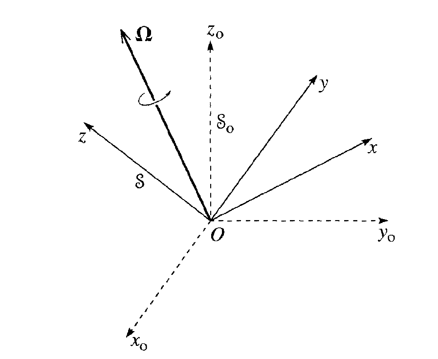
For a reference frame that rotates with respect to an inertial frame, Euler's theorem is central here. It states that the most general displacement (motion) of a rigid body with a one point fixed (we normally approximate a rigid body with a mass center) is a rotation about some fixed axis. In different words, the most general motion of any body relative to a fixed point \( O \) is a rotation abotu some axis through the same point \( O \). This means that for a specific rotation about a given point \( O \) we only to specify the direction of the axis about which the rotation occurs with the corresponding angle of rotation. As we will see below, the direction of the angle of rotation can be specified by a unit vector \( \boldsymbol{e} \) in the rotating frame and the rate of rotation per unit time. The latter defines the angular velocity \( \Omega \). We will define these quantities more rigorously below. At the end of this section we will also prove Euler's theorem.
What we will show here is that Newton's laws for an object in the rotating frame is given by $$ m\ddot{\boldsymbol{r}}_{S}=\boldsymbol{F}+m\boldsymbol{r}\times\dot{\boldsymbol{\Omega}}+2m\boldsymbol{v}_S\times\boldsymbol{\Omega}+m\left(\boldsymbol{\Omega}\times\boldsymbol{r}\right)\times\boldsymbol{\Omega}. $$
The first term to the right is the force we defined in the inertial system, that is \( m\ddot{\boldsymbol{r}}_{S_0}=\boldsymbol{F} \). The second term is the angular acceleration of the rotating reference frame, a quantity which in many cases is set to zero since we assume that the angular velocity is constant as function of time. The third terms is the Coriolis force, that is $$ \boldsymbol{F}_{\mathrm{Coriolis}}=2m\boldsymbol{v}_S\times\boldsymbol{\Omega}, $$ while the last term is going to give us the standard centrifugal force $$ \boldsymbol{F}_{\mathrm{Centrifugal}}=m\left(\boldsymbol{\Omega}\times\boldsymbol{r}\right)\times\boldsymbol{\Omega}. $$
Let us derive these terms, following much of the same procedure as we did for an accelerating reference frame. The figure here (to come) shows the two reference systems \( S \) and \( S_0 \).
We define a general vector \( \boldsymbol{A} \). It could represent the position, a given force, the velocity and other quantities of interest for studies of the equations of motion.
We let this vector to be defined by three orthogonal (we assume motion in three dimensions) unit vectors \( \boldsymbol{e}_i \), that is we have $$ \boldsymbol{A}=A_1\boldsymbol{e}_1+A_2\boldsymbol{e}_2+A_3\boldsymbol{e}_3=\sum_iA_i\boldsymbol{e}_i. $$
These unit vectors are fixed in the rotating frame, that is their time derivatives are zero. However, for an observer in the inertial frame \( S_0 \), however these unit vectors are rotating and may thus have an explicit time dependence.
Since we want to find an expression for the equations of motion in the inertial frame and the rotating frame, we need expressions for the time derivative of a vector \( \boldsymbol{A} \) in these two frames. Since the unit vectors are assumed to be fixed in \( S \), we have $$ \dot{\boldsymbol{A}}_S=\sum_i\frac{dA_i}{dt}\boldsymbol{e}_i=\sum_i\dot{dA_i}\boldsymbol{e}_i. $$
In the inertial frame \( S_0 \) we have $$ \dot{\boldsymbol{A}}_{S_0}=\sum_i\dot{dA_i}\boldsymbol{e}_i+\sum_i A_i\left(\dot{\boldsymbol{e}}_i\right)_{S_0}. $$
We will show below that $$ \left(\dot{\boldsymbol{e}}_i\right)_{S_0}=\Omega\times\boldsymbol{e}_i, $$
where \( \Omega \) is the angular velocity (to be derived below). This means we can write the derivative of an arbitrary vector \( \boldsymbol{A} \) in the inertial frame \( S_0 \) as (the vector is defined in the rotating frame), $$ \dot{\boldsymbol{A}}_{S_0}=\sum_i\dot{dA_i}\boldsymbol{e}_i+\sum_i A_i\left(\dot{\boldsymbol{e}}_i\right)_{S_0}=\dot{\boldsymbol{A}}_S+\sum_i A_i(\Omega\times\boldsymbol{e}_i)=\dot{\boldsymbol{A}}_S+\boldsymbol{\Omega}\times\boldsymbol{A}. $$
This is a very useful relation which relates the derivative of any vector \( \boldsymbol{A} \) measured in the inertial frame \( S_0 \) to the correspoding derivative in a rotating frame \( S \).
If we now let \( \boldsymbol{A} \) be the position and the velocity vectors, we can derive the equations of motion in the rotating frame in terms of the same equations of motion in the inertial frame \( S_0 \).
Let us start with the position \( \boldsymbol{r} \).
We have $$ \dot{\boldsymbol{r}}_{S_0}=\dot{\boldsymbol{r}}_S+\boldsymbol{\Omega}\times\boldsymbol{r}. $$
If we define the velocities in the two frames as $$ \boldsymbol{v}_{S_0}=\dot{\boldsymbol{r}}_{S_0}, $$ and $$ \boldsymbol{v}_{S}=\dot{\boldsymbol{r}}_{S}, $$ we have then $$ \dot{\boldsymbol{r}}_{S_0}=\boldsymbol{v}_{S_0}=\boldsymbol{v}_{S}+\boldsymbol{\Omega}\times\boldsymbol{r}. $$
In order to find the equations of motion, we need the acceleration and thereby the time derivative of the last equation. The derivative of the angular velocity \( \Omega \) will turn in handy in these derivations (repeated applications of the chain rule again). The latter derivative is $$ \dot{\boldsymbol{\Omega}}_{S_0}=\dot{\boldsymbol{\Omega}}_S+\boldsymbol{\Omega}\times\boldsymbol{\Omega}, $$
which leads to (an expected result, why?) $$ \dot{\boldsymbol{\Omega}}_{S_0}=\dot{\boldsymbol{\Omega}}_S, $$
since \( \boldsymbol{\Omega}\times\boldsymbol{\Omega}=0 \).
Let us now take the second derivative with respect to time.
Using $$ \left[\frac{d^2\boldsymbol{r}}{dt^2}\right]_{S_0}=\ddot{\boldsymbol{r}}_{S_0}=\left[\frac{d}{dt}\right]_{S_0}\left[\frac{d\boldsymbol{r}}{dt}\right]_{S_0}, $$
we have $$ \ddot{\boldsymbol{r}}_{S_0}=\left[\frac{d}{dt}\right]_{S_0}\left[\boldsymbol{v}_{S}+\boldsymbol{\Omega}\times\boldsymbol{r}\right]=\left[\frac{d}{dt}\right]_{S_0}\boldsymbol{v}_{S_0}, $$
which gives $$ \ddot{\boldsymbol{r}}_{S_0}=\left[\frac{d\boldsymbol{v}_S}{dt}\right]_{S}+\dot{\boldsymbol{\Omega}}\times \boldsymbol{r}+2\boldsymbol{\Omega}\times\boldsymbol{v}_S+\boldsymbol{\Omega}\times(\boldsymbol{\Omega}\times\boldsymbol{r}). $$
Defining the accelerations \( \boldsymbol{a}_{S_0}=\ddot{\boldsymbol{r}}_{S_0}=\dot{\boldsymbol{v}}_{S_0} \) and \( \boldsymbol{a}_{S}=\dot{\boldsymbol{v}}_{S} \), we have $$ \boldsymbol{a}_{S_0}=\boldsymbol{a}_{S}+\dot{\boldsymbol{\Omega}}\times \boldsymbol{r}+2\boldsymbol{\Omega}\times\boldsymbol{v}_S+\boldsymbol{\Omega}\times(\boldsymbol{\Omega}\times\boldsymbol{r}). $$
If we now use Newton's law in the inertial frame \( \boldsymbol{F}=m\boldsymbol{a}_{S_0} \), we get the effective force in the rotating frame (multiplying by the mass \( m \)) $$ m\boldsymbol{a}_{S}=\boldsymbol{F}+m\dot{\boldsymbol{r}\times\boldsymbol{\Omega}}+2m\boldsymbol{v}_S\times\boldsymbol{\Omega}+m(\boldsymbol{\Omega}\times\boldsymbol{r})\times\boldsymbol{\Omega}, $$ which is what we wanted to demostrate. We have the Coriolis force $$ \boldsymbol{F}_{\mathrm{Coriolis}}=2m\boldsymbol{v}_S\times\boldsymbol{\Omega}, $$ while the last term is the standard centrifugal force $$ \boldsymbol{F}_{\mathrm{Centrifugal}}=m\left(\boldsymbol{\Omega}\times\boldsymbol{r}\right)\times\boldsymbol{\Omega}. $$
In our discussions below we will assume that the angular acceleration of the rotating frame is zero and focus only on the Coriolis force and the centrifugal force.
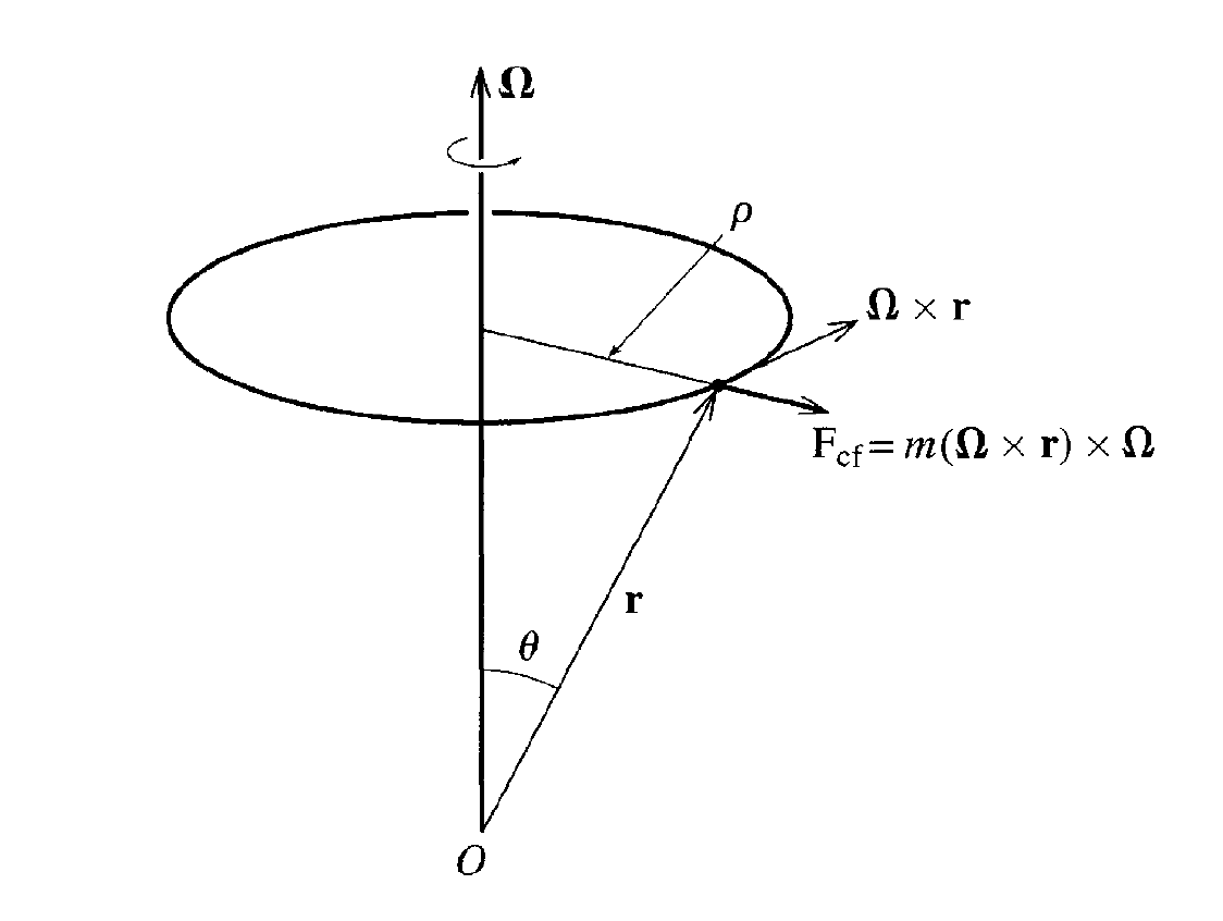
Suppose we can ignore the Coriolis force. If we focus only on the centrifugal force we have an additional force $$ \boldsymbol{F}_{\mathrm{Centrifugal}}=m\left(\boldsymbol{\Omega}\times\boldsymbol{r}\right)\times\boldsymbol{\Omega}, $$
where the term \( \boldsymbol{\Omega}\times\boldsymbol{r} \) is the radial velocity.
Consider now an object with position \( \boldsymbol{r} \) according to an observer in a frame rotating about the \( z \) axis with angular velocity \( \boldsymbol{\Omega}=\Omega\hat{z} \). To an observer in the inertial frame the vector will change even if the vector appears fixed to the rotating observer.
If \( \boldsymbol{\Omega} \) is in the \( z \) direction, the centrifugal force becomes $$ \begin{equation} \boldsymbol{F}_{\mathrm{Centrifugal}}=m\Omega^2(x\hat{x}+y\hat{y}). \label{_auto2} \end{equation} $$
The centrifugal force points outward in the \( x-y \) plane, and its magnitude is \( m\Omega^2r \), where \( r=\sqrt{x^2+y^2} \).
Continuing along these lines,
if we define a rotating frame which makes an angle \( \theta \) with the inertial frame and define the distance to an object in this frame from the origin as \( \boldsymbol{r} \), then the centrifugal force (which points outward) has as magnitude \( \Omega^2r\sin{\theta} \). Defining \( \rho=r\sin{\theta} \) and the unit vector \( \hat{\boldsymbol{\rho}} \) (see figure here)
If we now go back again to our falling object discussed in the beginning of these lectures, we need to modify for the fact that the Earth is rotating with respect to the falling object.
Seen from a rotating coordinate system we have now that the forces acting on the falling object are $$ m\ddot{\boldsymbol{r}}=\boldsymbol{F}_{\mathrm{gravity}}+\boldsymbol{F}_{\mathrm{Centrifugal}}. $$
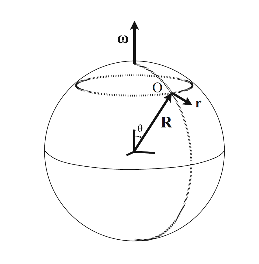
If we define the mass of Earth as \( M \) and its radius as \( R \) and assuming that the object is close to the Earth, the gravitational force takes then well-known expression $$ \boldsymbol{F}_{\mathrm{gravity}}=-\frac{GMm}{R^2}\hat{\boldsymbol{r}}=m\boldsymbol{g}_0. $$ Inserting the expression for the centrifugal force, we can then define an effective force $$ \boldsymbol{F}_{\mathrm{eff}}=\boldsymbol{F}_{\mathrm{gravity}}+\boldsymbol{F}_{\mathrm{Centrifugal}}=m\boldsymbol{g}_0-m\Omega^2R\sin{(\theta)}\hat{\boldsymbol{\rho}}, $$ and with $$ \boldsymbol{g}_{\mathrm{eff}}=\boldsymbol{g}_0-\Omega^2R\sin{(\theta)}\hat{\boldsymbol{\rho}}, $$ we have $$ \boldsymbol{F}_{\mathrm{eff}}=m\boldsymbol{g}_{\mathrm{eff}}. $$
In the rotating coordinate system (not an inertial frame), motion is thus determined by an apparent force and one can define effective potentials. In addition to the normal gravitational potential energy, there is a contribution to the effective potential, $$ \begin{equation} \delta V_{\rm eff}(r)=-\frac{m}{2}\Omega^2r^2=-\frac{m}{2}r^2\Omega^2\sin^2\theta, \label{_auto3} \end{equation} $$
where \( \theta \) is the polar angle, measured from say the north pole. If the true gravitational force can be considered as originating from a point in Earth's center, the net effective potential for a mass \( m \) near Earth's surface could be (a distance \( h \)) $$ \begin{equation} V_{\rm eff}=mgh-m\frac{1}{2}\Omega^2(R+h)^2\sin^2\theta. \label{_auto4} \end{equation} $$
As an example, let us ask ourselves how much wider is Earth at the equator than the north-south distance between the poles assuming that the gravitational field above the surface can be approximated by that of a point mass at Earth's center.
The surface of the ocean must be at constant effective potential for a sample mass \( m \). This means that if \( h \) now refers to the height of the water $$ m g[h(\theta=\pi/2)-h(\theta=0)]=\frac{m}{2}\Omega^2(R+h)^2. $$
Because \( R>>h \), one can approximate \( R+h\rightarrow R \) on the right-hand side, thus $$ h(\theta=\pi)-h(\theta=0)=\frac{\Omega^2R^2}{2g}. $$
This come out a bit less than 11 km, or a difference of near 22 km for the diameter of the Earth in the equatorial plane compared to a diameter between the poles. In reality, the difference is approximately 41 km. The discrepancy comes from the assumption that the true gravitational force can be treated as if it came from a point at Earth's center. This would be true if the distribution of mass was radially symmetric. However, Earth's center is molten and the rotation distorts the mass distribution. Remarkably this effect nearly doubles the elliptic distortion of Earth's shape. Due to this distortion, the top of Mount Everest is not the furthest point from the center of the Earth. That belongs to the top of a volcano, Chimborazo, in Equador, which is one degree in latitude below the Equator. Chimborazo is about 8500 ft lower than Everest when measured relative to sea level, but is 7700 feet further from the center of the Earth.
The Coriolis force is given by $$ \boldsymbol{F}_{\mathrm{Coriolis}}=2m\boldsymbol{v}_S\times\boldsymbol{\Omega}, $$
It does not enter problems like the shape of the Earth above because in that case the water was not moving relative to the rotating frame.
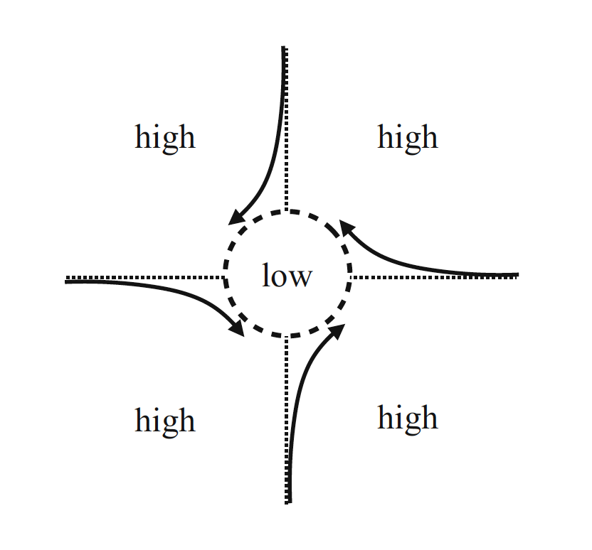
The Coriolis force is non-zero only if \( \boldsymbol{v}_S\ne 0 \) and is directed perpendicular to both \( \boldsymbol{v}_S \) and \( \Omega \). Viewed along the direction of \( \boldsymbol{v}_S \), the Coriolis force associated with counter-clockwise rotational motion produces a deflection to the right. For clockwise rotational motion, it produces a deflection to the left.
The Coriolis force associated with Earth’s rotational motion is
responsible for the circulating or cyclonic weather patterns
associated with hurricanes and cyclones, as illustrated in the figure
here. Basically, a pressure gradient gives rise to air currents that
tend to flow from high pressure to low pressure regions. But as the
air flows toward the low pressure region, the Coriolis force deflects
the air currents away from their straight line paths. Since the
projection of \( \Omega \) perpendicular to the local tangent plane
changes sign as one crosses the equator, the direction of the cyclonic
motion (either counter-clockwise or clockwise) is different in the
Northern and Southern hemispheres.
As an example, assume a ball is dropped from a height $h=500$m above Minneapolis. Due to the Coriolis force, it is deflected by an amount \( \delta x \) and \( \delta y \). We want to find the deflection due to the Coriolis force. Here we ignore the centrifugal terms.
The equations of motion are: $$ \begin{eqnarray*} \frac{dv_x}{dt}&=&-2(\Omega_yv_z-\Omega_zv_y),\\ \frac{dv_y}{dt}&=&-2(\Omega_zv_x-\Omega_xv_z),\\ \frac{dv_z}{dt}&=&-g-2(\Omega_xv_y-\Omega_yv_x),\\ \Omega_z&=&\Omega\cos\theta,~~~\Omega_y=\Omega\sin\theta,~~~\Omega_x=0. \end{eqnarray*} $$
Here the coordinate system is \( \hat{x} \) and points east, \( \hat{y} \) points north and \( \hat{z} \) points upward.
One can now ignore all the Coriolis terms on the right-hand sides except for those with \( v_z \). The other terms will all be doubly small. One can also throw out terms with \( \Omega_x \). This gives $$ \begin{eqnarray*} \frac{dv_x}{dt}&\approx& -2\Omega v_z\sin\theta,\\ \frac{dv_y}{dt}&\approx& 0,\\ \frac{dv_z}{dt}&\approx& -g. \end{eqnarray*} $$
There will be no significant deflection in the \( y \) direction, \( \delta y=0 \), but in the \( x \) direction one can substitute \( v_z=-gt \) above, $$ \begin{eqnarray*} v_x&\approx&\int_0^t dt'~2\Omega gt'\sin\theta=\Omega gt^2\sin\theta,\\ \delta x&\approx& \int_0^t dt'~v_x(t')=\frac{g\Omega\sin\theta t^3}{3}. \end{eqnarray*} $$
One can find the deflections by using \( h=\frac{1}{2}gt^2 \), to find the time, and using the all-knowing internet to see that the latitude of Minneapolis is \( 44.6^\circ \) or \( \theta=45.4^\circ \). $$ \begin{eqnarray*} t&=&\sqrt{2h/g}=10.1~{\rm s},\\ \Omega&=&\frac{2\pi}{3600\cdot 24~{\rm s}}=7.27\times 10^{-5}~{\rm s}^{-1},\\ \delta x&=&17.4~{\rm cm}~~{\rm(east)}. \end{eqnarray*} $$
It is now simple to bring together the equations for an accelerating and rotating frame. Using our results we have the equations of motion for an object in an accelerating and rotating frame with respect to an inertial frame $$ m\ddot{\boldsymbol{r}}_{S}=\boldsymbol{F}+m\boldsymbol{r}\times\dot{\boldsymbol{\Omega}}+2m\boldsymbol{v}_S\times\boldsymbol{\Omega}+m\left(\boldsymbol{\Omega}\times\boldsymbol{r}\right)\times\boldsymbol{\Omega}-\boldsymbol{a}_{S_0}, $$ where the last term is the acceleration of the accelerating frame seen from the inertial frame.
The Foucault Pendulum is simply a regular pendulum moving in both horizontal directions, and with the Coriolis force included. It is explained at its simplest if we consider a pendulum positioned at the North pole. Foucault's experiment was actually the first laboratory demonstration that the Earth is rotating. The experiment is rather simple and many physics department worldwide have their own pendulum.
In the original experiment done in Paris in 1851, Foucault used a massive pendulum of 28kg and 67m long.
If use an inertial frame with the North pole as its origin, the Earth below the pendulum rotates with a period of 24h (actually 23h and 56min). Seen with respect to the surface of the Earth, the plane of the pendulum moves in the opposite direction of the rotation of the Earth.
If we were to perform the experiment in other places, the setup is slightly more complicated since the pendulum will then rotate with the Earth. The net effect is a slower rotation compared to North pole.
Let us look at the equations we need to solve. $$ \begin{eqnarray*} m\ddot{\boldsymbol{r}}&=&\boldsymbol{T}+m\boldsymbol{g}-2m\boldsymbol{\Omega}\times\boldsymbol{v}, \end{eqnarray*} $$
as the centrifugal force term is absorbed into the definition of \( \boldsymbol{g} \). The magnitude of the tension, \( \boldsymbol{T} \), is considered constant because we consider only small oscillations. Then \( T\approx mg \), and the components, using \( \hat{x},\hat{y} \) to correspond to east and north respectively, are $$ \begin{eqnarray*} T_x=-mgx/L,~~~T_y=-mgy/L. \end{eqnarray*} $$
If \( \Omega \) is the rotation of the earth, and if \( \theta \) is the polar angle, \( \pi \)-latitude, $$ \begin{eqnarray*} \ddot{x}&=&-gx/L+2\dot{y}\Omega_z,\\ \ddot{y}&=&-gy/L-2\dot{x}\Omega_z. \end{eqnarray*} $$
Here we have used the fact that the oscillations are sufficiently small so we can ignore \( v_z \). Using \( \Omega_0\equiv\sqrt{k/m} \), $$ \begin{eqnarray*} \ddot{x}-2\Omega_z\dot{y}+\Omega_0^2x&=&0\\ \ddot{y}+2\Omega_z\dot{x}+\Omega_0^2y&=&0, \end{eqnarray*} $$
where \( \Omega_z=|\boldsymbol{\Omega}|\cos\theta \), with \( \theta \) being the polar angle (zero at the north pole). The terms linear in time derivatives are what make life difficult. This will be solved with a trick. We will incorporate both differential equations into a single complex equation where the first/second are the real/imaginary parts. $$ \begin{eqnarray*} \eta\equiv x+iy,\\ \ddot{\eta}+2i\Omega_z\dot{\eta}+\Omega_0^2\eta&=&0. \end{eqnarray*} $$
Now, we guess at a form for the solutions, \( \eta(t)=e^{-i\alpha t} \), which turns the differential equation into $$ \begin{eqnarray*} -\alpha^2+2\Omega_z\alpha+\Omega_0^2&=&0,\\ \alpha&=&\Omega_z\pm \sqrt{\Omega_z^2+\Omega_0^2},\\ &\approx&\Omega_z\pm \Omega_0. \end{eqnarray*} $$
The solution with two arbitrary constants is then $$ \begin{eqnarray*} \eta&=&e^{-i\Omega_zt}\left[C_1e^{i\Omega_0t}+C_2e^{-i\Omega_0t}\right]. \end{eqnarray*} $$
Here, \( C_1 \) and \( C_2 \) are complex, so they actually represent four arbitrary numbers. These four numbers should be fixed by the four initial conditions, i.e. \( x(t=0), \dot{x}(t=0), y(t=0) \) and \( \dot{y}(t=0) \). With some lengthy algebra, one can rewrite the expression as $$ \begin{eqnarray*} \label{eq:precmess} \eta&=&e^{-i\Omega_zt}\left[A\cos(\Omega_0t+\phi_A)+iB\cos(\Omega_0t+\phi_B)\right]. \end{eqnarray*} $$
Here, the four coefficients are represented by the two real arbitrary real amplitudes, \( A \) and \( B \), and two arbitrary phases, \( \phi_A \) and \( \phi_B \). For an initial condition where \( y=0 \) at \( t=0 \), one can see that \( B=0 \). This then gives $$ \begin{eqnarray*} \eta(t)&=&Ae^{-i\Omega_zt}\cos(\Omega_0t+\gamma)\\ \nonumber &=&A\cos\Omega_zt\cos(\Omega_0t+\gamma)+iA\sin\Omega_zt\cos(\Omega_0t+\gamma). \end{eqnarray*} $$
Translating into \( x \) and \( y \), $$ \begin{eqnarray} x&=&A\cos\Omega_zt\cos(\Omega_0t+\gamma),\\ \nonumber y&=&A\sin\Omega_zt\cos(\Omega_0t+\gamma). \end{eqnarray} $$
Assuming the pendulum's frequency is much higher than Earth's rotational frequency, \( \Omega_0>>\Omega_z \), one can see that the plane of the pendulum simply precesses with angular velocity \( \Omega_z \). This means that in this limit the pendulum oscillates only in the \( x \)-direction with frequency many times before the phase \( \Omega_zt \) becomes noticeable. Eventually, when \( \Omega_zt=\pi/2 \), the motion is along the \( y \)-direction. If you were at the north pole, the motion would switch from the \( x \)-direction to the \( y \) direction every 6 hours. Away from the north pole, \( \Omega_z\ne|\boldsymbol{\Omega}| \) and the precession frequency is less. At the equator it does not precess at all. If one were to repeat for the solutions where \( A=0 \) and \( B\ne 0 \), one would look at motions that started in the \( y \)-direction, then precessed toward the \( -x \) direction. Linear combinations of the two sets of solutions give pendulum motions that resemble ellipses rather than simple back-and-forth motion.
this material will be added soon